Build gauge charts with Kibana
Elastic Cloud Serverless projects are autoscaled environments, fully managed by Elastic and available on Elastic Cloud. Availability This functionality is generally available and ready for production usage. Serverless interfaces and procedures might differ from classic Elastic Stack deployments. The Elastic Stack includes Elastic's core products such as Elasticsearch, Kibana, Logstash, and Beats. Availability This functionality is generally available and ready for production usage. Unless stated otherwise on the page, this functionality is available when your Elastic Stack is deployed on Elastic Cloud Hosted, Elastic Cloud Enterprise, Elastic Cloud on Kubernetes, and self-managed environments. This documentation corresponds to the latest patch available for each minor version. If you're not using the latest patch, check the release notes for changes.
Serverless
Generally available
Stack
Generally available
Gauge charts display a single value within a defined range, showing how close the value is to a target or threshold. They are ideal for monitoring KPIs, tracking progress toward goals, and highlighting when values fall within acceptable, warning, or critical ranges. Unlike metric charts that display raw values, gauge charts add range context with known minimum and maximum boundaries.
You can build a gauge chart in Kibana in either of these ways:
To automate chart or dashboard creation, use the Dashboards and Visualizations APIs. To create dashboards from natural-language instructions, use Elastic Agent Builder or the Kibana dashboards agent skill.
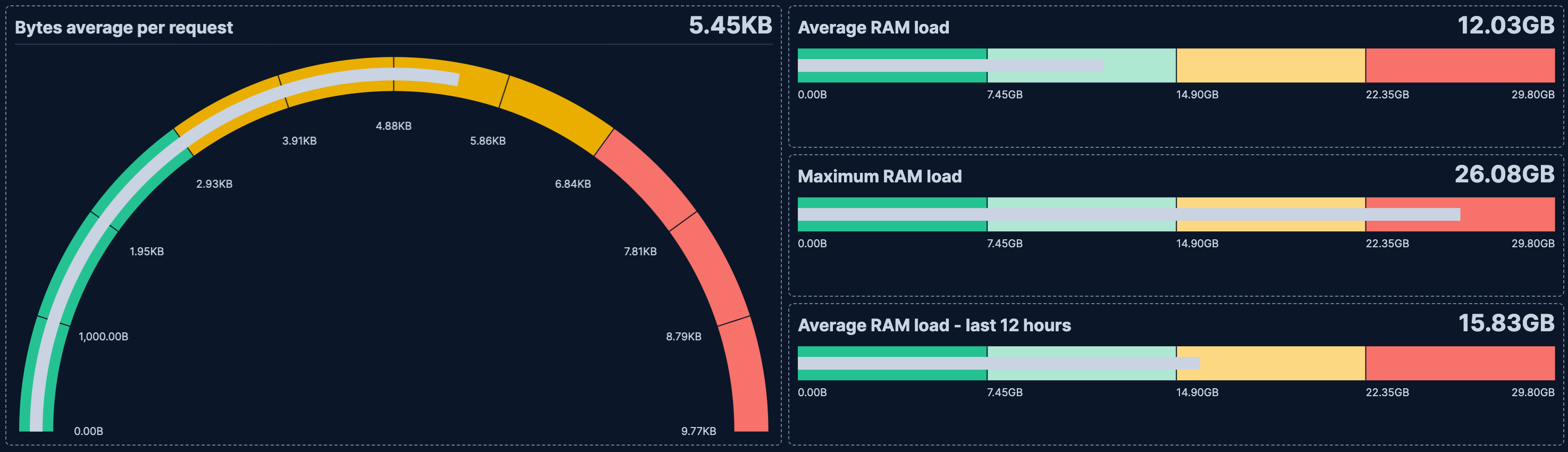
Before you start, make sure you have data indexed into Elasticsearch or install sample data. The point-and-click editor uses data views to access your Elasticsearch data. Data views are usually created automatically when you ingest data. You can also create one manually to select the data that you want.
To build a gauge chart:
-
Lens is Kibana's main visualization editor. You can access it:
- From a dashboard: On the Dashboards page, open or create the dashboard where you want to add the visualization, then add a new visualization.
- From the Visualize library, by opening it and creating a new visualization.
-
New visualizations often start as Bar charts.
Using the Visualization type dropdown, select Gauge.
-
- Select the data view that contains your data.
- Configure the Metric dimension to define the value displayed on the gauge.
Optionally:
- Configure the Minimum value dimension to set the lower bound of the gauge range.
- Configure the Maximum value dimension to set the upper bound of the gauge range.
- Configure the Goal dimension to display a target marker on the gauge.
Each of these optional dimensions can be set as a static number, computed dynamically from your data using an aggregation, or defined with a formula.
The chart preview updates to show a gauge with your metric value positioned within the range. If the gauge appears empty, verify that the selected field contains numeric data for the current time range.
-
- If you accessed Lens from a dashboard, select Save and return to save the visualization and add it to that dashboard, or select Save to library to add the visualization to the Visualize library and be able to add it to other dashboards later.
- If you accessed Lens from the Visualize library, select Save. A menu opens and lets you add the visualization to a dashboard and to the Visualize library.
Before you start, make sure you have data indexed into Elasticsearch or install sample data. ES|QL queries the indices named in the query directly, so you do not need a data view. The columns returned by the query become available as chart dimensions. Refer to Visualizations using ES|QL queries to learn how to open the editor, shape the query result for a visualization, and save the visualization.
A gauge chart needs a single numeric metric to position its indicator within the configured range. In this query, STATS has no BY clause, so it reduces all matching documents to one row containing the average number of bytes per request:
FROM kibana_sample_data_logs
| STATS average_bytes = AVG(bytes)
To build the chart:
- Create an ES|QL visualization and run the query.
- Set the visualization type to Gauge.
- Assign
average_bytesto the Metric dimension. - Set value ranges that give the metric context.
- Customize the chart appearance using the gauge chart settings.
- Select Apply and close.
The chart preview shows where the average number of bytes falls within the configured ranges.
After building the chart with the point-and-click editor or an ES|QL query, customize its appearance for your data and audience:
- Set meaningful bounds
- Define the minimum and maximum values that make sense for your metric. A CPU usage gauge should range from 0 to 100, while a sales target might range from 0 to your quarterly goal.
- Use color bands for thresholds
- Configure color ranges to indicate performance levels. Use green for acceptable values, yellow for warning, and red for critical thresholds.
- Choose the right shape
- Select a gauge shape that fits your dashboard layout. Use Arc shapes for traditional gauge appearance, or Linear for a more compact horizontal or vertical display.
- Add context with titles
- Provide clear titles that explain what the gauge measures and what the target value represents.
Refer to Gauge chart settings for all gauge chart configuration options. For panel sizing and layout guidance, refer to Organize dashboard panels.
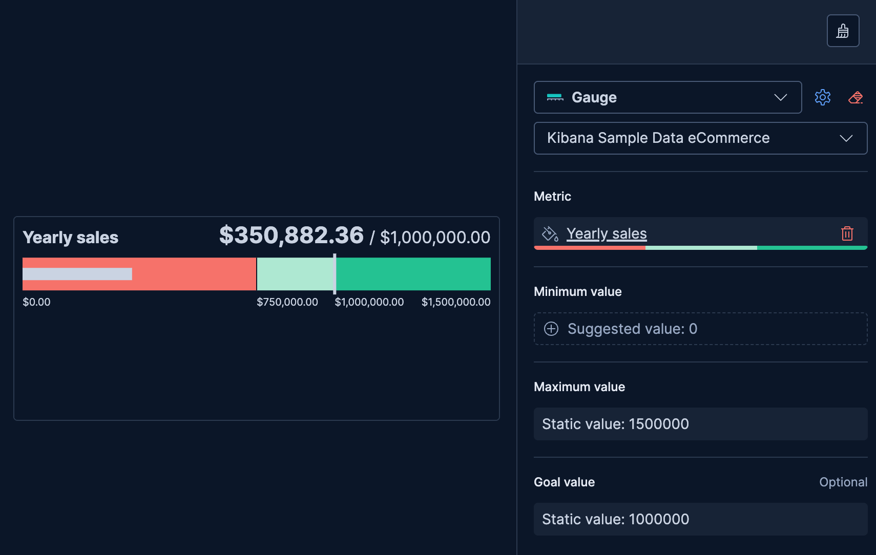
Use a gauge to track progress toward a specific target, such as monthly sales goals or project completion percentage.
- Create a Gauge chart and select your data view.
- Configure the Metric dimension with your progress value (for example,
Sum(sales_amount)). - Configure the Minimum value dimension as a static value of
0. - Configure the Maximum value dimension as a static value matching your target (for example,
100000for a $100K sales goal). - Configure the Goal dimension as a static value matching your target to display a goal marker on the gauge.
- Select the Metric dimension, enable Band colors, and configure Color mapping with bands to show progress levels.
Serverless Stack GA 9.5+ … Create this chart using the API
This example creates a horizontal bullet gauge that sums order revenue from the eCommerce sample data, providing a quick view of progress toward a sales goal.
These API request examples are kept up to date with the latest version of the APIs, so some fields might differ if you're using an earlier version. For a history of breaking changes, refer to the Kibana breaking changes or the Elastic Cloud Serverless breaking changes.
POST kbn://api/visualizations{ "type": "gauge", "title": "Yearly sales goal", "filters": [], "query": { "expression": "" }, "styling": { "shape": { "type": "bullet", "orientation": "horizontal" } }, "metric": { "operation": "sum", "field": "products.taxful_price", "empty_as_null": true, "label": "Yearly sales", "max": { "operation": "static_value", "value": 1500000 }, "goal": { "operation": "static_value", "value": 1000000 }, "title": { "visible": true }, "ticks": { "visible": true, "mode": "bands" }, "color": { "type": "dynamic", "range": "absolute", "steps": [ { "gte": 0, "lt": 750000, "color": "#f6726a" }, { "gte": 750000, "lt": 1000000, "color": "#aee8d2" }, { "gte": 1000000, "color": "#24c292" } ] } }, "data_source": { "type": "data_view_spec", "index_pattern": "kibana_sample_data_ecommerce", "time_field": "order_date" } }
bulletwithorientation: "horizontal"renders a compact linear bar gauge, ideal for placing multiple KPIs in a row.sumofproducts.taxful_pricetracks cumulative revenue as the gauge metric.maxsets the upper bound of the scale (1.5M) andgoalplaces a target marker at 1M, so progress toward the goal is immediately visible. The threestepscolor bands turn the bar red below 750K, light green approaching the goal, and green once it's reached.
curl -X POST "${KIBANA_URL}/api/visualizations" \
  -H "Authorization: ApiKey ${API_KEY}" \
  -H "kbn-xsrf: true" \
  -H "Content-Type: application/json" \
  -d '{
  "type": "gauge",
  "title": "Yearly sales goal",
  "filters": [],
  "query": { "expression": "" },
  "styling": {
    "shape": { "type": "bullet", "orientation": "horizontal" }
  },
  "metric": {
    "operation": "sum",
    "field": "products.taxful_price",
    "empty_as_null": true,
    "label": "Yearly sales",
    "max": { "operation": "static_value", "value": 1500000 },
    "goal": { "operation": "static_value", "value": 1000000 },
    "title": { "visible": true },
    "ticks": { "visible": true, "mode": "bands" },
    "color": {
      "type": "dynamic",
      "range": "absolute",
      "steps": [
        { "gte": 0, "lt": 750000, "color": "#f6726a" },
        { "gte": 750000, "lt": 1000000, "color": "#aee8d2" },
        { "gte": 1000000, "color": "#24c292" }
      ]
    }
  },
  "data_source": {
    "type": "data_view_spec",
    "index_pattern": "kibana_sample_data_ecommerce",
    "time_field": "order_date"
  }
}'
bulletwithorientation: "horizontal"renders a compact linear bar gauge, ideal for placing multiple KPIs in a row.sumofproducts.taxful_pricetracks cumulative revenue as the gauge metric.maxsets the upper bound of the scale (1.5M) andgoalplaces a target marker at 1M, so progress toward the goal is immediately visible. The threestepscolor bands turn the bar red below 750K, light green approaching the goal, and green once it's reached.
For more information, refer to the Visualizations API.
Color bands help users quickly understand whether a value is within acceptable ranges.
- Create a Gauge chart with your metric configured.
- Select the Metric dimension to open its settings.
- Enable Band colors.
- In Color mapping, select a color palette (or use the default Status palette) and adjust the band boundaries and colors.
- Optionally, enable Ticks on bands to display tick marks at the band boundaries on the gauge scale.
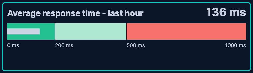
This example shows a gauge with server response time and color-coded health indicators.
| Band | Range | Color | Meaning |
|---|---|---|---|
| Healthy | 0-200ms | Green | Normal response times |
| Warning | 200-500ms | Light green | Elevated response times |
| Critical | 500ms+ | Red | Unacceptable performance |
Serverless Stack GA 9.5+ … Create this chart using the API
This example creates a gauge with three color-coded threshold bands so the arc turns green, yellow, or red depending on the average byte count.
These API request examples are kept up to date with the latest version of the APIs, so some fields might differ if you're using an earlier version. For a history of breaking changes, refer to the Kibana breaking changes or the Elastic Cloud Serverless breaking changes.
POST kbn://api/visualizations{ "type": "gauge", "title": "Server response time", "filters": [], "query": { "expression": "" }, "styling": { "shape": { "type": "bullet", "orientation": "horizontal" } }, "metric": { "operation": "median", "field": "memory", "label": "Average response time - last hour", "format": { "type": "duration", "from": "us", "to": "ms" }, "min": { "operation": "static_value", "value": 0 }, "max": { "operation": "formula", "formula": "1000000" }, "title": { "visible": true }, "ticks": { "visible": true, "mode": "bands" }, "color": { "type": "dynamic", "range": "absolute", "steps": [ { "color": "#24c292", "gte": 0, "lt": 200000 }, { "color": "#aee8d2", "gte": 200000, "lt": 500000 }, { "color": "#f6726a", "gte": 500000 } ] } }, "data_source": { "type": "data_view_spec", "index_pattern": "kibana_sample_data_logs", "time_field": "timestamp" } }
color.type: "dynamic"applies color bands based on the metric value, giving instant visual feedback on health status.- Each
stepsentry defines a range and color: green for healthy (0–200ms), light green for warning (200–500ms), and red for critical (500ms+). Thedurationformat converts raw microsecond values to human-readable milliseconds.
curl -X POST "${KIBANA_URL}/api/visualizations" \
  -H "Authorization: ApiKey ${API_KEY}" \
  -H "kbn-xsrf: true" \
  -H "Content-Type: application/json" \
  -d '{
  "type": "gauge",
  "title": "Server response time",
  "filters": [],
  "query": { "expression": "" },
  "styling": { "shape": { "type": "bullet", "orientation": "horizontal" } },
  "metric": {
    "operation": "median",
    "field": "memory",
    "label": "Average response time - last hour",
    "format": { "type": "duration", "from": "us", "to": "ms" },
    "min": { "operation": "static_value", "value": 0 },
    "max": { "operation": "formula", "formula": "1000000" },
    "title": { "visible": true },
    "ticks": { "visible": true, "mode": "bands" },
    "color": {
      "type": "dynamic",
      "range": "absolute",
      "steps": [
        { "color": "#24c292", "gte": 0, "lt": 200000 },
        { "color": "#aee8d2", "gte": 200000, "lt": 500000 },
        { "color": "#f6726a", "gte": 500000 }
      ]
    }
  },
  "data_source": {
    "type": "data_view_spec",
    "index_pattern": "kibana_sample_data_logs",
    "time_field": "timestamp"
  }
}'
color.type: "dynamic"applies color bands based on the metric value, giving instant visual feedback on health status.- Each
stepsentry defines a range and color: green for healthy (0–200ms), light green for warning (200–500ms), and red for critical (500ms+). Thedurationformat converts raw microsecond values to human-readable milliseconds.
For more information, refer to the Visualizations API.
Instead of entering fixed static values, you can use fields from your data to set the minimum, maximum, or goal dynamically using aggregations.
- Create a Gauge chart with your metric configured.
- In the Maximum value dimension, select a field and aggregation that represents the upper bound (for example,
Max(quota)for a quota-based gauge). - Optionally, do the same for Minimum value (for example,
Min(baseline)) or Goal (for example,Average(target)).
This approach is useful when bounds or targets vary by category, time period, or user. You can also use formulas to define dynamic bounds or goals. Refer to Lens formulas for more details.
Customize your gauge chart to display exactly the information you need, formatted the way you want.
The Metric dimension defines the main value displayed on the gauge.
- Data
-
The value that the gauge displays. When you drag a field onto the chart, Kibana suggests a function based on the field type. You can use aggregation functions like
Sum,Average,Count,Median,Last value, and more, or create custom calculations with formulas.Advanced settings
Depending on the data you defined, several options allow you to apply additional filtering to the data taken into account to compute the final value to show.
Based on the type of visualization you're creating, only some of the following options can be available:
- Normalize by unit: Normalize the metric values to show per unit of time.
- Filter by: Specify a query.
- Reduced time range: Reduce the time range specified on the dashboard's time filter by the specified duration.
- Time shift: Shift the time range by the specified duration. This is useful if the value should use a different time range than the one selected on the dashboard.
- Hide zero values: Don't show values equal to zero. This option is on by default.
- Appearance
-
- Name: Customize the metric label displayed in the gauge.
- Value format: Control how numeric values are displayed (number, percent, bytes, and more).
- Band colors: Toggle to enable colored bands on the gauge. When enabled, the following options appear:
- Color mapping: Configure the color palette and define color stops for the bands. The default palette is Status with 4 color steps.
- Ticks on bands: Toggle to place tick marks at band boundaries instead of distributing them evenly along the gauge scale.
The Minimum value dimension defines the lower bound of the gauge range.
- Data
-
Set a static value, use a field with an aggregation like
Min, or create a custom calculation with a formula. When adding this dimension, you can enter a fixed number directly (static value) or select a field to compute the minimum dynamically. If not configured, the gauge infers a minimum from the data.Advanced settings
Depending on the data you defined, several options allow you to apply additional filtering to the data taken into account to compute the final value to show.
Based on the type of visualization you're creating, only some of the following options can be available:
- Normalize by unit: Normalize the metric values to show per unit of time.
- Filter by: Specify a query.
- Reduced time range: Reduce the time range specified on the dashboard's time filter by the specified duration.
- Time shift: Shift the time range by the specified duration. This is useful if the value should use a different time range than the one selected on the dashboard.
- Hide zero values: Don't show values equal to zero. This option is on by default.
NoteThe minimum value must be less than the maximum value. If the minimum is greater than or equal to the maximum, the gauge displays an error.
- Appearance
-
- Name: Customize the label for the minimum value.
The Maximum value dimension defines the upper bound of the gauge range.
- Data
-
Set a static value, use a field with an aggregation like
Max, or create a custom calculation with a formula. When adding this dimension, you can enter a fixed number directly (static value) or select a field to compute the maximum dynamically. If not configured, the gauge infers a maximum from the data.Advanced settings
Depending on the data you defined, several options allow you to apply additional filtering to the data taken into account to compute the final value to show.
Based on the type of visualization you're creating, only some of the following options can be available:
- Normalize by unit: Normalize the metric values to show per unit of time.
- Filter by: Specify a query.
- Reduced time range: Reduce the time range specified on the dashboard's time filter by the specified duration.
- Time shift: Shift the time range by the specified duration. This is useful if the value should use a different time range than the one selected on the dashboard.
- Hide zero values: Don't show values equal to zero. This option is on by default.
- Appearance
-
- Name: Customize the label for the maximum value.
The Goal dimension displays a target marker on the gauge, providing a visual reference point for the metric value.
- Data
-
Set a static value, use a field with an aggregation, or create a custom calculation with a formula. When adding this dimension, you can enter a fixed number directly (static value) or select a field to compute the goal dynamically. The goal marker appears as a line or indicator on the gauge scale.
Advanced settings
Depending on the data you defined, several options allow you to apply additional filtering to the data taken into account to compute the final value to show.
Based on the type of visualization you're creating, only some of the following options can be available:
- Normalize by unit: Normalize the metric values to show per unit of time.
- Filter by: Specify a query.
- Reduced time range: Reduce the time range specified on the dashboard's time filter by the specified duration.
- Time shift: Shift the time range by the specified duration. This is useful if the value should use a different time range than the one selected on the dashboard.
- Hide zero values: Don't show values equal to zero. This option is on by default.
- Appearance
-
- Name: Customize the label for the goal value.
When creating or editing a visualization, you can customize several appearance options from the Style menu.
- Shape
-
Choose the gauge shape:
- Linear: A bar gauge, displayed horizontally (default) or vertically. Select Horizontal or Vertical orientation after choosing this shape.
- Minor arc: A partial circle arc.
- Major arc: A larger circular arc.
- Circle: A full 360-degree gauge.
Titles and text
- Title
-
Control the gauge title:
- Auto: Display the metric name automatically (default).
- Custom: Enter a custom title.
- None: Hide the title.
- Subtitle
-
Add an optional subtitle for additional context:
- Custom: Enter a custom subtitle.
- None: No subtitle (default).
The following examples show various configuration options for building impactful gauge charts.
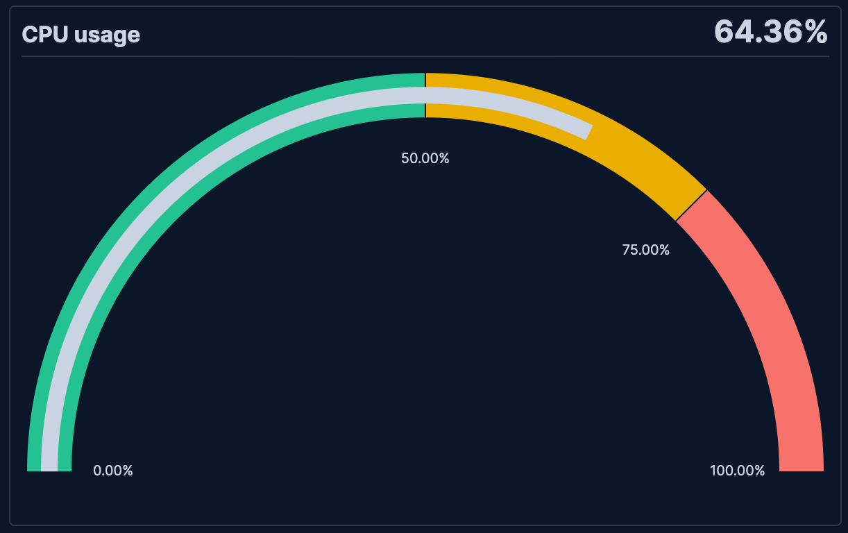
- CPU usage monitoring
-
Monitor system CPU usage with threshold-based coloring:
- Example based on: Kibana Sample Data Logs
- Metric: Formula
average(machine.ram)/20000000000formatted as percent - Maximum: Formula
max(machine.ram)/32211000000 - Shape: Semi-circle
- Color bands: 0–50% (green), 50–75% (yellow), 75%+ (red)
Serverless Stack GA 9.5+ … Create this chart using the API
This example creates a CPU-monitoring gauge with green/yellow/red threshold bands, using machine.ram from the logs sample data as a proxy for a CPU-like metric.
These API request examples are kept up to date with the latest version of the APIs, so some fields might differ if you're using an earlier version. For a history of breaking changes, refer to the Kibana breaking changes or the Elastic Cloud Serverless breaking changes.
POST kbn://api/visualizations{ "type": "gauge", "title": "CPU usage", "filters": [], "query": { "expression": "" }, "styling": { "shape": { "type": "semi_circle" } }, "metric": { "operation": "formula", "formula": "average(machine.ram)/20000000000", "label": "CPU usage", "format": { "type": "percent", "decimals": 2, "compact": false }, "max": { "operation": "formula", "formula": "max(machine.ram)/32211000000" }, "title": { "visible": true }, "ticks": { "visible": true, "mode": "bands" }, "color": { "type": "dynamic", "range": "percentage", "steps": [ { "gte": 0, "lt": 50, "color": "#24c292" }, { "gte": 50, "lt": 75, "color": "#EAAE01" }, { "gte": 75, "color": "#f6726a" } ] } }, "data_source": { "type": "data_view_spec", "index_pattern": "kibana_sample_data_logs", "time_field": "timestamp" } }
formulacomputes the ratio of average RAM to a reference value, producing a 0–1 ratio formatted as a percentage. Replace with your actual CPU metric field (for example,average(system.cpu.total.pct)).range: "percentage"maps the color thresholds proportionally across the gauge's 0–100% scale: green below 50%, yellow between 50–75%, and red above 75%.
curl -X POST "${KIBANA_URL}/api/visualizations" \
  -H "Authorization: ApiKey ${API_KEY}" \
  -H "kbn-xsrf: true" \
  -H "Content-Type: application/json" \
  -d '{
  "type": "gauge",
  "title": "CPU usage",
  "filters": [],
  "query": { "expression": "" },
  "styling": { "shape": { "type": "semi_circle" } },
  "metric": {
    "operation": "formula",
    "formula": "average(machine.ram)/20000000000",
    "label": "CPU usage",
    "format": { "type": "percent", "decimals": 2, "compact": false },
    "max": { "operation": "formula", "formula": "max(machine.ram)/32211000000" },
    "title": { "visible": true },
    "ticks": { "visible": true, "mode": "bands" },
    "color": {
      "type": "dynamic",
      "range": "percentage",
      "steps": [
        { "gte": 0, "lt": 50, "color": "#24c292" },
        { "gte": 50, "lt": 75, "color": "#EAAE01" },
        { "gte": 75, "color": "#f6726a" }
      ]
    }
  },
  "data_source": {
    "type": "data_view_spec",
    "index_pattern": "kibana_sample_data_logs",
    "time_field": "timestamp"
  }
}'
formulacomputes the ratio of average RAM to a reference value, producing a 0–1 ratio formatted as a percentage. Replace with your actual CPU metric field (for example,average(system.cpu.total.pct)).range: "percentage"maps the color thresholds proportionally across the gauge's 0–100% scale: green below 50%, yellow between 50–75%, and red above 75%.
For more information, refer to the Visualizations API.
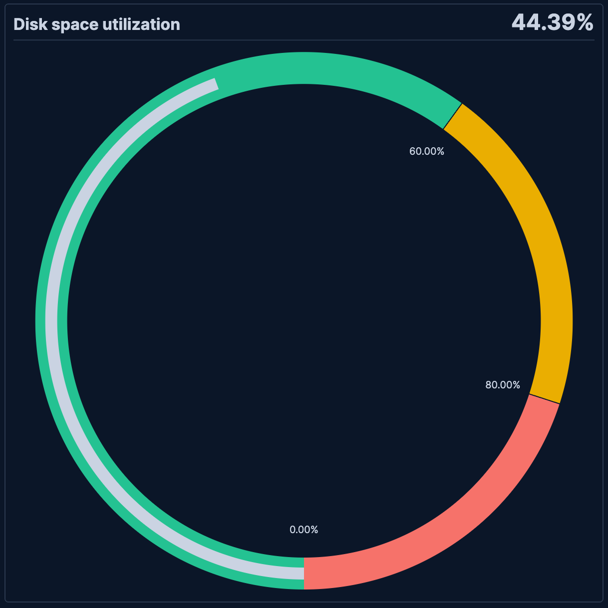
- Disk space utilization
-
Display disk space usage as a percentage of capacity:
- Example based on: Kibana Sample Data Logs
- Metric: Formula
average(machine.ram)/29000000000formatted as percent - Maximum: Formula
max(machine.ram)/32211000000 - Shape: Circle
- Color bands: 0–60% (green), 60–80% (yellow), 80%+ (red)
Serverless Stack GA 9.5+ … Create this chart using the API
This example creates a full-circle disk utilization gauge with color bands that shift from green to red as usage increases, using machine.ram from the logs sample data as a proxy.
These API request examples are kept up to date with the latest version of the APIs, so some fields might differ if you're using an earlier version. For a history of breaking changes, refer to the Kibana breaking changes or the Elastic Cloud Serverless breaking changes.
POST kbn://api/visualizations{ "type": "gauge", "title": "Disk space utilization", "filters": [], "query": { "expression": "" }, "styling": { "shape": { "type": "circle" } }, "metric": { "operation": "formula", "formula": "average(machine.ram)/29000000000", "label": "Disk space utilization", "format": { "type": "percent", "decimals": 2, "compact": false }, "max": { "operation": "formula", "formula": "max(machine.ram)/32211000000" }, "title": { "visible": true }, "ticks": { "visible": true, "mode": "bands" }, "color": { "type": "dynamic", "range": "percentage", "steps": [ { "gte": 0, "lt": 60, "color": "#24c292" }, { "gte": 60, "lt": 80, "color": "#EAAE01" }, { "gte": 80, "color": "#f6726a" } ] } }, "data_source": { "type": "data_view_spec", "index_pattern": "kibana_sample_data_logs", "time_field": "timestamp" } }
circledraws a full 360-degree gauge, which works well for utilization percentages where the full range is always visible.- The
formuladivides average RAM by a reference capacity value to produce a 0–1 ratio formatted as percent. Replace with your actual disk metric (for example,sum(system.filesystem.used.bytes) / sum(system.filesystem.total.bytes)). - The
percentagerange maps thresholds proportionally: green below 60%, yellow between 60–80%, and red above 80%, so the gauge turns red only when disk usage becomes critical.
curl -X POST "${KIBANA_URL}/api/visualizations" \
  -H "Authorization: ApiKey ${API_KEY}" \
  -H "kbn-xsrf: true" \
  -H "Content-Type: application/json" \
  -d '{
  "type": "gauge",
  "title": "Disk space utilization",
  "filters": [],
  "query": { "expression": "" },
  "styling": {
    "shape": { "type": "circle" }
  },
  "metric": {
    "operation": "formula",
    "formula": "average(machine.ram)/29000000000",
    "label": "Disk space utilization",
    "format": { "type": "percent", "decimals": 2, "compact": false },
    "max": { "operation": "formula", "formula": "max(machine.ram)/32211000000" },
    "title": { "visible": true },
    "ticks": { "visible": true, "mode": "bands" },
    "color": {
      "type": "dynamic",
      "range": "percentage",
      "steps": [
        { "gte": 0, "lt": 60, "color": "#24c292" },
        { "gte": 60, "lt": 80, "color": "#EAAE01" },
        { "gte": 80, "color": "#f6726a" }
      ]
    }
  },
  "data_source": {
    "type": "data_view_spec",
    "index_pattern": "kibana_sample_data_logs",
    "time_field": "timestamp"
  }
}'
circledraws a full 360-degree gauge, which works well for utilization percentages where the full range is always visible.- The
formuladivides average RAM by a reference capacity value to produce a 0–1 ratio formatted as percent. Replace with your actual disk metric (for example,sum(system.filesystem.used.bytes) / sum(system.filesystem.total.bytes)). - The
percentagerange maps thresholds proportionally: green below 60%, yellow between 60–80%, and red above 80%, so the gauge turns red only when disk usage becomes critical.
For more information, refer to the Visualizations API.