Learn data exploration and visualization with Kibana

Kibana provides powerful tools for exploring and visualizing data stored in Elasticsearch. Discover lets you search and filter documents with Elasticsearch Query Language (ES|QL), Lens transforms query results into charts, and Dashboards combine visualizations into shareable, interactive views. This tutorial teaches you how these core features work together by walking through a complete workflow, from querying data to sharing a finished dashboard.

You'll use Kibana's built-in sample web logs dataset so you can focus on learning the tools without needing to set up data ingestion. Basic familiarity with Elasticsearch concepts (indices, documents, fields) is helpful but not required.

These features are available across all Elastic solutions and project types, so what you learn here applies regardless of your use case.

By the end of this tutorial, you'll know how to:

Search, filter, and aggregate data in Discover using ES|QL
Create visualizations with Lens
Combine panels into a Dashboard and customize the layout
Navigate between Discover, Lens, and Dashboards to iterate on your analysis
Share a dashboard with your team

Before you begin

An Elastic Stack deployment or Elastic Cloud Serverless project with Elasticsearch and Kibana. Don't have one yet? Start a free trial.
The required privileges to complete the tutorial. Specifically:
- Kibana privileges: All on Discover and Dashboard (to explore data and create dashboards).
- Elasticsearch index privileges: read and view_index_metadata on the kibana_sample_data_logs index (to query the sample data in Discover).
Note

If you created a trial account, you are the admin of your deployment and already have all the required privileges.

Step 1: Load sample data

Before you can explore and visualize, you need data in Elasticsearch. In this tutorial you use Kibana's built-in sample web logs dataset, which you can load in a few clicks. No agents or integrations required.

Open the Integrations page from the navigation menu or using the global search field.
In the list of integrations, select Sample Data.
Install the Sample web logs data set:
- Elastic Cloud Serverless projects are autoscaled environments, fully managed by Elastic and available on Elastic Cloud. Availability Generally available This functionality is generally available and ready for production usage. Serverless interfaces and procedures might differ from classic Elastic Stack deployments. The Elastic Stack includes Elastic's core products such as Elasticsearch, Kibana, Logstash, and Beats. Availability Generally available since 9.4 This functionality is generally available and ready for production usage. Unless stated otherwise on the page, this functionality is available when your Elastic Stack is deployed on Elastic Cloud Hosted, Elastic Cloud Enterprise, Elastic Cloud on Kubernetes, and self-managed environments. This documentation corresponds to the latest patch available for each minor version. If you're not using the latest patch, check the release notes for changes. On the Sample web logs card, select Install data.
- The Elastic Stack includes Elastic's core products such as Elasticsearch, Kibana, Logstash, and Beats. Availability Generally available from 9.0 to 9.3 This functionality is generally available and ready for production usage. Unless stated otherwise on the page, this functionality is available when your Elastic Stack is deployed on Elastic Cloud Hosted, Elastic Cloud Enterprise, Elastic Cloud on Kubernetes, and self-managed environments. This documentation corresponds to the latest patch available for each minor version. If you're not using the latest patch, check the release notes for changes. Select Other sample data sets, then on the Sample web logs card, select Add data.

The sample data is loaded into the kibana_sample_data_logs index. It includes web server access logs with fields like @timestamp, clientip, response, bytes, url, extension, and geo.src.

Tip

When you're ready to explore your own data, refer to Ingest data for an overview of ingestion options, including Elastic Agent, Beats, and direct API uploads. Many integrations also ship with pre-built dashboards, visualizations, anomaly detection jobs, and alerting rules, so you can start analyzing your data as soon as it's ingested.

Step 2: Explore data in Discover with ES|QL

Discover is the starting point for data exploration. You can search, filter, and visualize your data interactively.

Discover supports two exploration modes. This tutorial uses ES|QL (Elasticsearch Query Language), a piped query language that lets you chain operations like filtering, aggregating, and sorting in a single query. Unlike classic mode, ES|QL doesn't require you to set up a data view first: you query your data sources directly by name, so you can start exploring right away.

Open Discover in ES|QL mode
1. From the navigation menu, go to Discover.
2. If Discover doesn't open in ES|QL mode, select Query in ES|QL (Try ES|QL in earlier Elastic Stack versions) in the application menu.
Result: Discover is in ES|QL mode, with an editor where you can write piped queries.
Run your first query

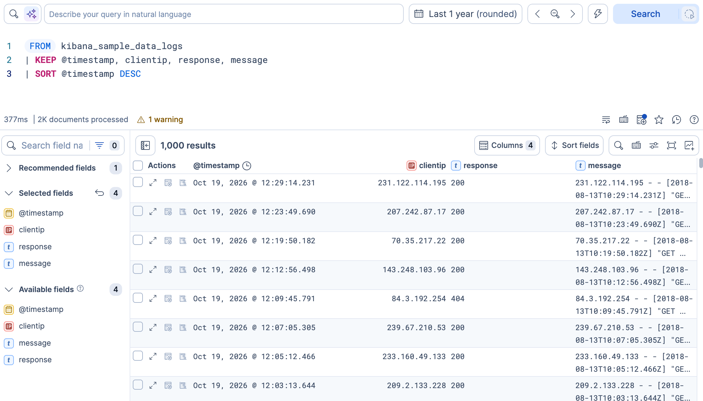
Enter the following query, then select Run or Search. If you choose to type your own query, the editor helps you with relevant autocomplete suggestions for commands, fields, and values.
ES|QL
```
FROM kibana_sample_data_logs
| KEEP @timestamp, clientip, response, message
| SORT @timestamp DESC
```
1. Reads from the sample web logs index.
2. Retains only these four fields in the output, discarding everything else.
3. Orders results by timestamp, most recent first.
You can add more ES|QL commands and functions to control the results of the query. For example, a | LIMIT command to cap the number of rows returned (the default is 1,000). Refer to the ES|QL reference for the full list of commands.

Result: The results table displays the most recent web log entries with only the fields you selected. Because the query uses KEEP, Discover doesn't show the chart of results over time. Instead, it shows a chart based on the columns you keep only when those columns suit one, so it's normal if no chart appears. To discover which fields are available, browse the field list in the sidebar.

Tip

No results? The time range filter defaults to the last 15 minutes. Sample data timestamps are relative to when you loaded the dataset, so you may need to select a wider range, such as Last 90 days, or more, to see results.
Inspect individual results and documents

The results table gives you an overview, but sometimes you need the full details of a single event. To inspect a document:
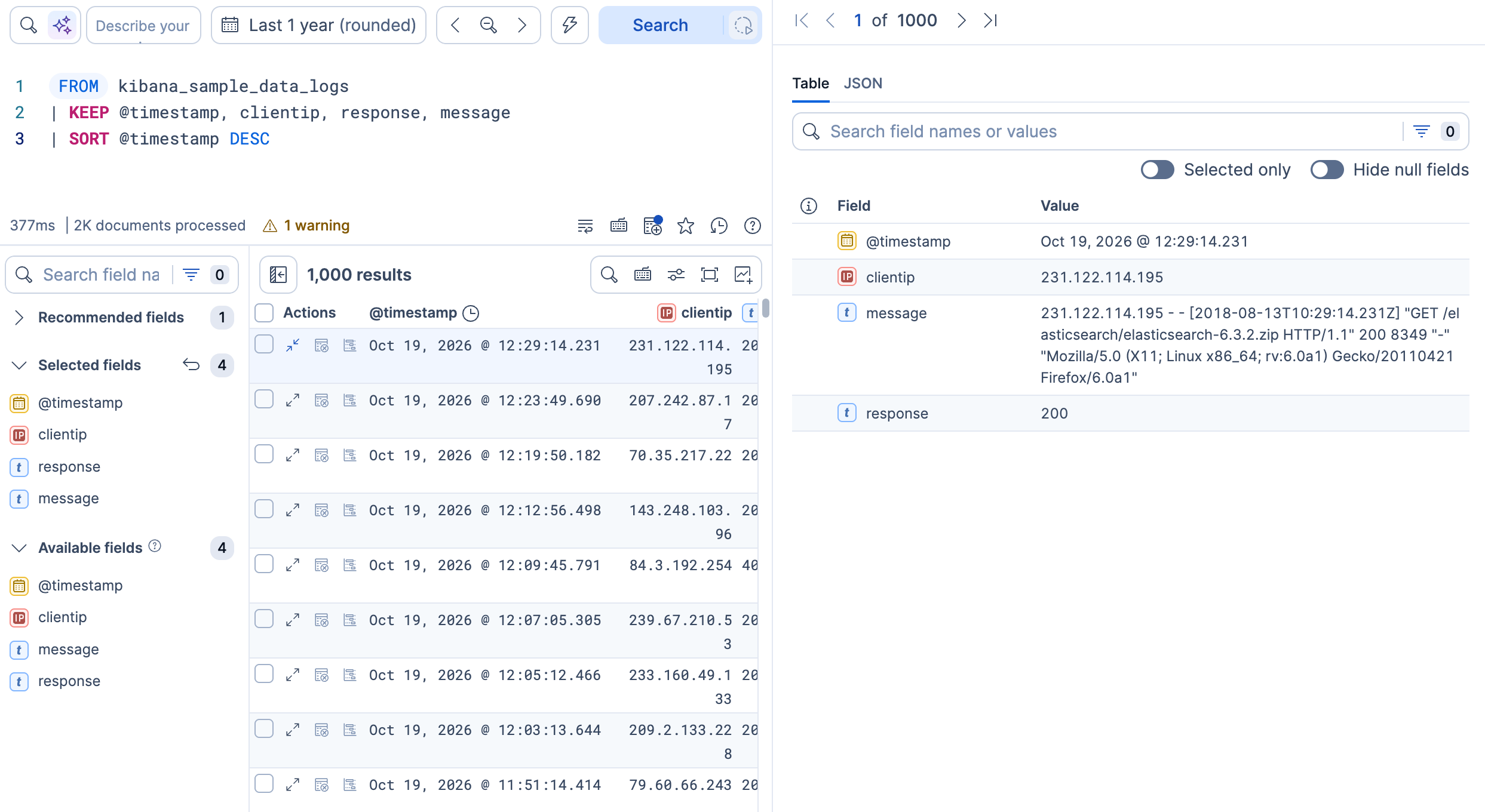
1. Select View details (Toggle dialog with details in earlier Elastic Stack versions) on any row in the results table. A flyout opens.
2. The flyout shows the fields returned by your query in a detailed view. Use the Table tab to see field names and values, or the JSON tab to see the raw document.
3. Use the navigation arrows at the top of the flyout to move between documents without closing it. This is useful when you need to compare consecutive events or trace a sequence.
Filter and aggregate

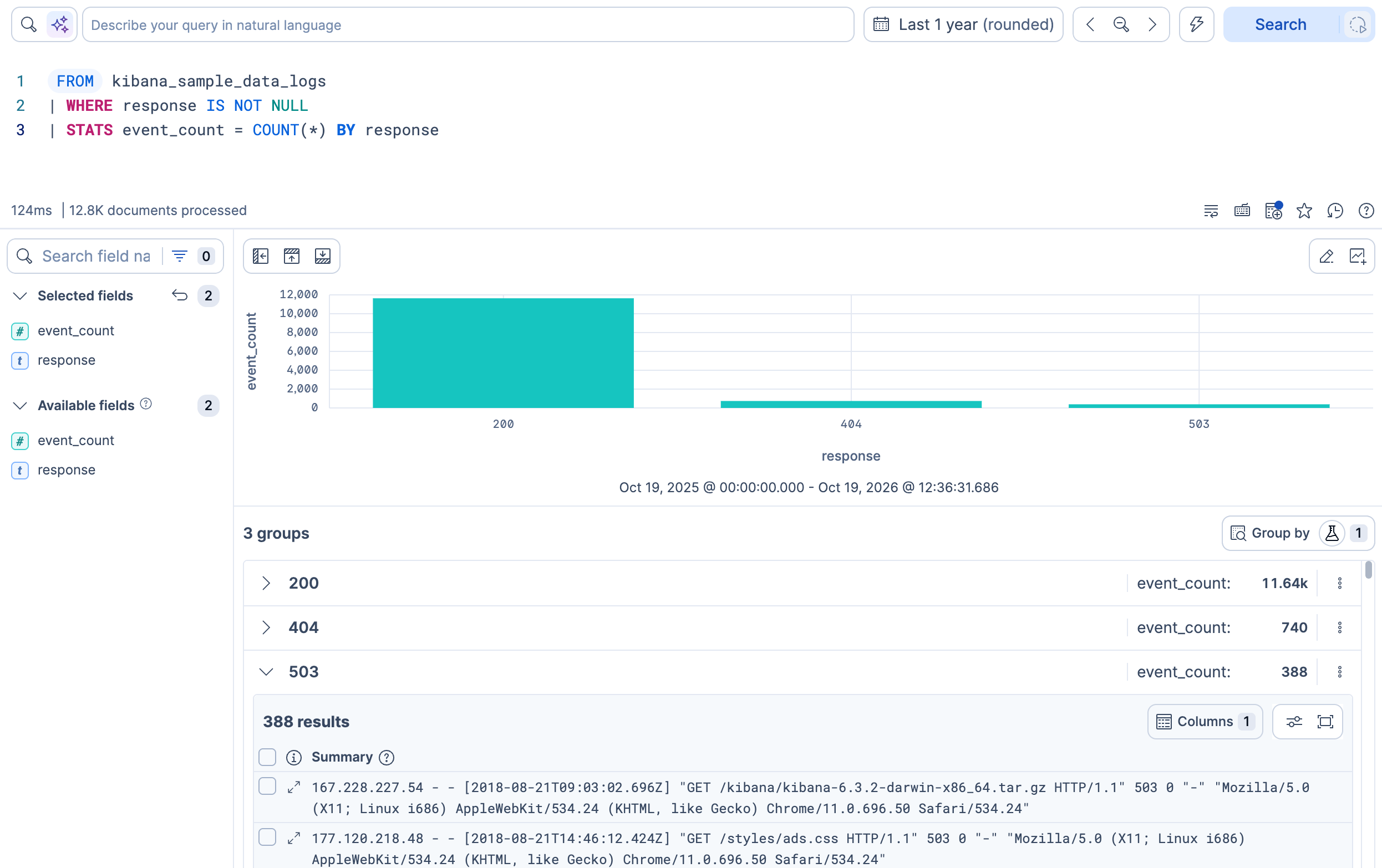
Browsing individual events is useful, but you can also summarize data directly in ES|QL. In this step, you check which HTTP response codes appear in the logs and how frequently. Use WHERE to filter out rows with missing values and STATS to count events per response code:
ES|QL
```
FROM kibana_sample_data_logs
| WHERE response IS NOT NULL
| STATS event_count = COUNT(*) BY response
```
1. Excludes rows where the HTTP response code is missing.
2. Groups rows by response code and counts events in each group.
Result: The table lists each HTTP response code with its event count. A chart appears above the table to visualize the aggregation, so you can see at a glance how traffic breaks down by status (200, 404, 503, and so on). A three-line query turned thousands of raw log entries into a breakdown with a chart. Notice that the field list in the sidebar now only shows the fields produced by the query (event_count and response), reflecting the narrower result set.

Elastic Cloud Serverless projects are autoscaled environments, fully managed by Elastic and available on Elastic Cloud. Availability Preview This functionality is in technical preview and is ready for evaluation. Use with caution in production; it is not recommended for mission-critical workloads. Elastic will work to fix any issues, but features in technical preview are not subject to the support SLA of official GA features. Specific Support terms apply. Serverless interfaces and procedures might differ from classic Elastic Stack deployments. The Elastic Stack includes Elastic's core products such as Elasticsearch, Kibana, Logstash, and Beats. Availability Preview since 9.4 This functionality is in technical preview and is ready for evaluation. Use with caution in production; it is not recommended for mission-critical workloads. Elastic will work to fix any issues, but features in technical preview are not subject to the support SLA of official GA features. Specific Support terms apply. Unless stated otherwise on the page, this functionality is available when your Elastic Stack is deployed on Elastic Cloud Hosted, Elastic Cloud Enterprise, Elastic Cloud on Kubernetes, and self-managed environments. This documentation corresponds to the latest patch available for each minor version. If you're not using the latest patch, check the release notes for changes. Instead of a flat table, Discover shows each response code as a group that you can expand to see the documents behind it. To return to a flat table, open the Group by menu and select none. Refer to Inspect grouped STATS results in Discover.
Save the visualization to a dashboard

The aggregation query produced a chart showing event counts by response code. You can save this chart directly to a dashboard:
1. Select Save visualization to dashboard (or Save visualization in earlier versions) next to the chart. You can also select Edit visualization to open the Lens editor inline and customize the chart before saving it.
2. Enter a title, for example Events by response code.
3. Under Add to dashboard, select New.
4. Select Save and go to dashboard.
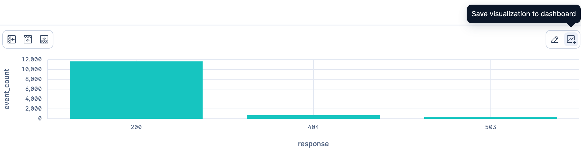
Result: Kibana opens a new, unsaved dashboard with your response code chart already on it. The chart is saved to the library and linked to the dashboard, so any edits you make to the chart are reflected on every dashboard that uses it. Panels you add directly to a dashboard without saving to the library are local to that dashboard only.

Tip

Want to show the results table on a dashboard instead of the chart? Save your Discover session (select Save in the toolbar), then from your dashboard, import it from the library as a new panel. This embeds the table view, including the query and any filters you applied.

You've queried, filtered, aggregated, and inspected data, all within Discover using ES|QL. You also saved a visualization to a new dashboard, which is where you're headed next. When you work with specific types of data, Discover adapts its interface accordingly. For example, it provides specialized log exploration tools with built-in parsing and categorization when it detects log data. To learn more about Discover, refer to Discover. For the full ES|QL language reference, refer to ES|QL.

Step 3: Build your dashboard

Now that you have a dashboard with your first panel, add more visualizations to tell a complete story about your web traffic.

Save the dashboard

Before adding more panels, save your dashboard so you don't lose your work:
1. In the toolbar, select Save.
2. Enter a title, for example Web logs overview.
3. Select Save.
Add a metric panel for median response size
1. Create the visualization:
  - Elastic Cloud Serverless projects are autoscaled environments, fully managed by Elastic and available on Elastic Cloud. Availability Generally available This functionality is generally available and ready for production usage. Serverless interfaces and procedures might differ from classic Elastic Stack deployments. The Elastic Stack includes Elastic's core products such as Elasticsearch, Kibana, Logstash, and Beats. Availability Generally available since 9.2 This functionality is generally available and ready for production usage. Unless stated otherwise on the page, this functionality is available when your Elastic Stack is deployed on Elastic Cloud Hosted, Elastic Cloud Enterprise, Elastic Cloud on Kubernetes, and self-managed environments. This documentation corresponds to the latest patch available for each minor version. If you're not using the latest patch, check the release notes for changes. Select Add → Create visualization (Visualization in earlier versions) in the toolbar.
  - The Elastic Stack includes Elastic's core products such as Elasticsearch, Kibana, Logstash, and Beats. Availability Generally available from 9.0 to 9.1 This functionality is generally available and ready for production usage. Unless stated otherwise on the page, this functionality is available when your Elastic Stack is deployed on Elastic Cloud Hosted, Elastic Cloud Enterprise, Elastic Cloud on Kubernetes, and self-managed environments. This documentation corresponds to the latest patch available for each minor version. If you're not using the latest patch, check the release notes for changes. Select Create visualization.
2. Make sure the Kibana Sample Data Logs data view is selected. If another one is selected, switch to Kibana Sample Data Logs so the fields in the next steps are available.
3. Once in the Lens editor, switch the visualization type to Metric.
4. From the Available fields list on the left, drag bytes to the Primary metric area. Lens selects the Median aggregation automatically.
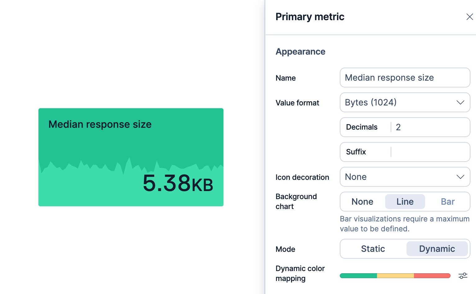
5. Select the "Median of bytes" Primary metric that we just added, then go to the Appearance section and configure the following:
  - Name: Median response size
  - Value format: Bytes (1024)
  - Background chart (or Supporting visualization): Line. A sparkline appears behind the number, showing how the median changes over the selected time range.
  - Mode (Color mode or Color by value in earlier versions): Dynamic. Set three color stops: green at 0, yellow at 6000, and red at 10000. With these thresholds, the panel color reflects whether the median response size is small (under 6 KB), moderate, or large (over 10 KB).
1. Select Close, then select Save and return.
Result: A metric panel appears on the dashboard showing the median response size in a human-readable format (for example, 5.6 KB instead of 5,748), with a background sparkline for context.
Optional: add more metrics to build a row
A dashboard often starts with a row of metrics for key numbers at a glance. Using the same steps, you can create additional metrics such as:
- Unique visitors: drag clientip. Lens picks Unique count for IP fields.
- Total requests: drag Records. Lens creates a simple count. To add a trend indicator, drag Records again to the Secondary metric area and set its Time shift to 1d. Then set Color mode (Color by value in earlier versions) to Dynamic and Compare to to Primary metric to show whether traffic is trending up or down. For details, refer to Show trends in Metric charts.
- Unique URLs: drag request.keyword. Lens picks Unique count, showing how many distinct pages were requested.
Add a line chart of log volume over time
1. Create the visualization:
  - Elastic Cloud Serverless projects are autoscaled environments, fully managed by Elastic and available on Elastic Cloud. Availability Generally available This functionality is generally available and ready for production usage. Serverless interfaces and procedures might differ from classic Elastic Stack deployments. The Elastic Stack includes Elastic's core products such as Elasticsearch, Kibana, Logstash, and Beats. Availability Generally available since 9.2 This functionality is generally available and ready for production usage. Unless stated otherwise on the page, this functionality is available when your Elastic Stack is deployed on Elastic Cloud Hosted, Elastic Cloud Enterprise, Elastic Cloud on Kubernetes, and self-managed environments. This documentation corresponds to the latest patch available for each minor version. If you're not using the latest patch, check the release notes for changes. Select Add → Create visualization (Visualization in earlier versions) in the toolbar.
  - The Elastic Stack includes Elastic's core products such as Elasticsearch, Kibana, Logstash, and Beats. Availability Generally available from 9.0 to 9.1 This functionality is generally available and ready for production usage. Unless stated otherwise on the page, this functionality is available when your Elastic Stack is deployed on Elastic Cloud Hosted, Elastic Cloud Enterprise, Elastic Cloud on Kubernetes, and self-managed environments. This documentation corresponds to the latest patch available for each minor version. If you're not using the latest patch, check the release notes for changes. Select Create visualization.
2. Once in the Lens editor, switch the visualization type to Line.
3. From the Available fields list, drag Records to the workspace.
  
  Because the data contains a time field, Lens places @timestamp on the horizontal axis and Count of Records on the vertical axis automatically.
4. From the Available fields list, drag host.keyword to the Breakdown area. Lens draws one line per host, each in a different color, so you can compare traffic patterns across servers.
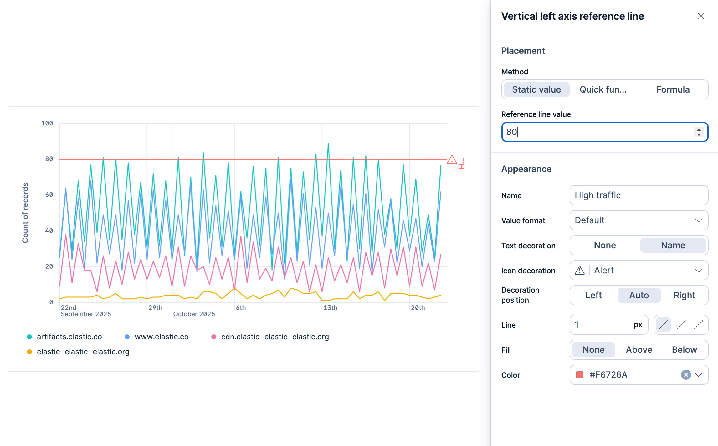
5. Add a reference line to give the chart visual context:
  1. Select the Add layer icon , then select Reference lines.
  2. Select the reference line value and enter 80. This marks a "high traffic" threshold on the chart. The value is only an example, so you can enter a different one.
  3. Set the color to red. In Name, enter a label such as High traffic, then set Text decoration to Name.
1. Select Save and return.
Add a panel title:
1. Hover over the panel and select Settings.
2. In the Title field, enter Log volume over time per host, then select Apply.
Optional: add more time series

To compare trends, create additional time series. For example, create a Response size over time per host panel: drag bytes to a new Line panel, then drag host.keyword to the Breakdown area to see how response sizes vary per host.
Add a bar chart of requests by file extension
1. Create the visualization:
  - Elastic Cloud Serverless projects are autoscaled environments, fully managed by Elastic and available on Elastic Cloud. Availability Generally available This functionality is generally available and ready for production usage. Serverless interfaces and procedures might differ from classic Elastic Stack deployments. The Elastic Stack includes Elastic's core products such as Elasticsearch, Kibana, Logstash, and Beats. Availability Generally available since 9.2 This functionality is generally available and ready for production usage. Unless stated otherwise on the page, this functionality is available when your Elastic Stack is deployed on Elastic Cloud Hosted, Elastic Cloud Enterprise, Elastic Cloud on Kubernetes, and self-managed environments. This documentation corresponds to the latest patch available for each minor version. If you're not using the latest patch, check the release notes for changes. Select Add → Create visualization (Visualization in earlier versions) in the toolbar.
  - The Elastic Stack includes Elastic's core products such as Elasticsearch, Kibana, Logstash, and Beats. Availability Generally available from 9.0 to 9.1 This functionality is generally available and ready for production usage. Unless stated otherwise on the page, this functionality is available when your Elastic Stack is deployed on Elastic Cloud Hosted, Elastic Cloud Enterprise, Elastic Cloud on Kubernetes, and self-managed environments. This documentation corresponds to the latest patch available for each minor version. If you're not using the latest patch, check the release notes for changes. Select Create visualization.
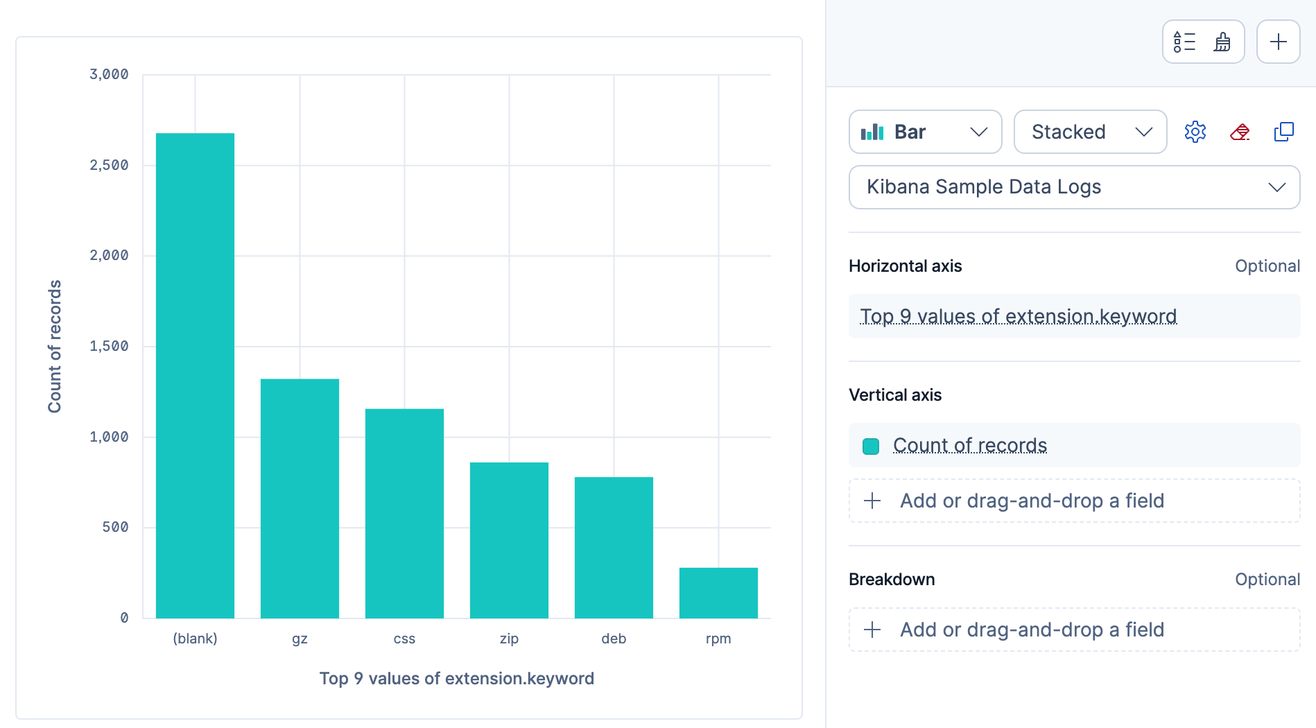
2. Make sure the correct data view is selected (for example, kibana_sample_data_logs).
3. From the Available fields list, drag extension.keyword to the workspace.
  
  Lens detects that this is a categorical field and creates a bar chart of its top values by count. It picks the chart type and axis configuration automatically.
1. Select Save and return.
Add a panel title:
1. Hover over the panel and select Settings. The Settings flyout appears.
2. In the Title field, enter Requests by file extension, then select Apply.
Result: A bar chart appears on the dashboard showing the most common file extensions by request count.
Add a table of recent events with ES|QL

You can also add panels powered by ES|QL queries directly from the dashboard. This is useful when you want to display raw events or run a specific query without going through Discover first.
1. Add a new panel:
  - Elastic Cloud Serverless projects are autoscaled environments, fully managed by Elastic and available on Elastic Cloud. Availability Generally available This functionality is generally available and ready for production usage. Serverless interfaces and procedures might differ from classic Elastic Stack deployments. The Elastic Stack includes Elastic's core products such as Elasticsearch, Kibana, Logstash, and Beats. Availability Generally available since 9.2 This functionality is generally available and ready for production usage. Unless stated otherwise on the page, this functionality is available when your Elastic Stack is deployed on Elastic Cloud Hosted, Elastic Cloud Enterprise, Elastic Cloud on Kubernetes, and self-managed environments. This documentation corresponds to the latest patch available for each minor version. If you're not using the latest patch, check the release notes for changes. Select Add in the application menu, then select Create visualization (query) (Visualization (query) or New panel → ES|QL under Visualizations in earlier versions).
  - The Elastic Stack includes Elastic's core products such as Elasticsearch, Kibana, Logstash, and Beats. Availability Generally available from 9.0 to 9.1 This functionality is generally available and ready for production usage. Unless stated otherwise on the page, this functionality is available when your Elastic Stack is deployed on Elastic Cloud Hosted, Elastic Cloud Enterprise, Elastic Cloud on Kubernetes, and self-managed environments. This documentation corresponds to the latest patch available for each minor version. If you're not using the latest patch, check the release notes for changes. Select Add panel in the application menu, then select ES|QL under Visualizations.
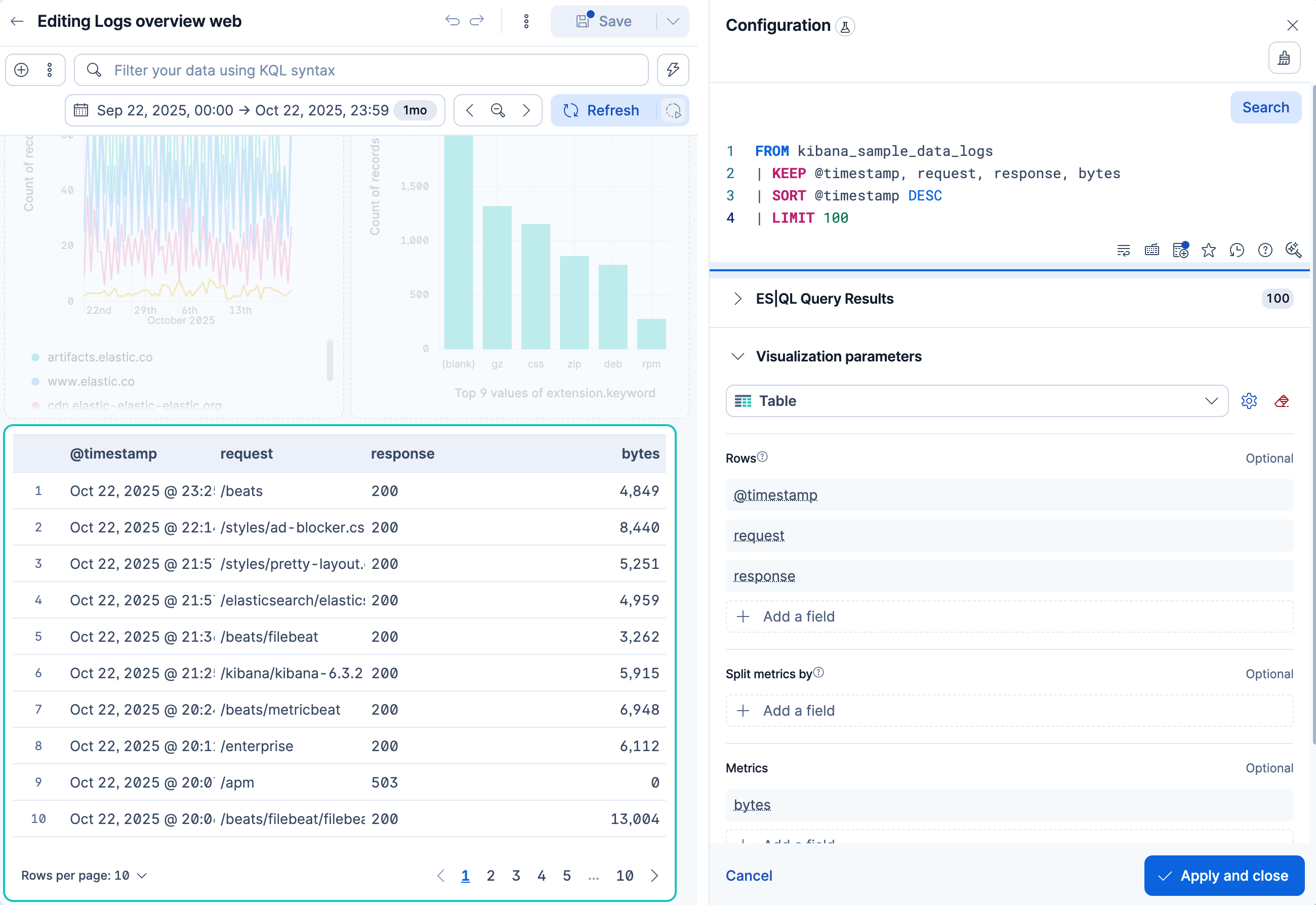
2. Enter the following query and run it:
  ES|QL
```
FROM kibana_sample_data_logs
| KEEP @timestamp, request, response, bytes
| SORT @timestamp DESC
| LIMIT 100
```
  1. Selects only the columns you want in the table.
  2. Shows the most recent events first.
  3. Caps the table at 100 records.
3. In the visualization type dropdown, select Table.
4. In the styling options, enable Paginate table so the panel stays compact on the dashboard while still giving access to all rows.
1. Select Apply and close.
Result: Your dashboard now has at least five panels: the response code chart from Discover, the metric, the line chart, the bar chart, and the ES|QL table, plus any additional panels you may have created from the optional suggestions.
Expand your dashboard

Lens supports many visualization types beyond metrics, lines, bars, and tables. To keep building your dashboard, you can add panels such as:
- A pie chart of traffic distribution by operating system (machine.os.keyword).
- A treemap breaking down requests by geography (geo.dest).
Each one follows the same workflow you have used so far: create a visualization, pick a type, drag fields, and save.
Customize a panel with inline editing

You can fine-tune any Lens panel without leaving the dashboard. Try it on the Requests by file extension panel:
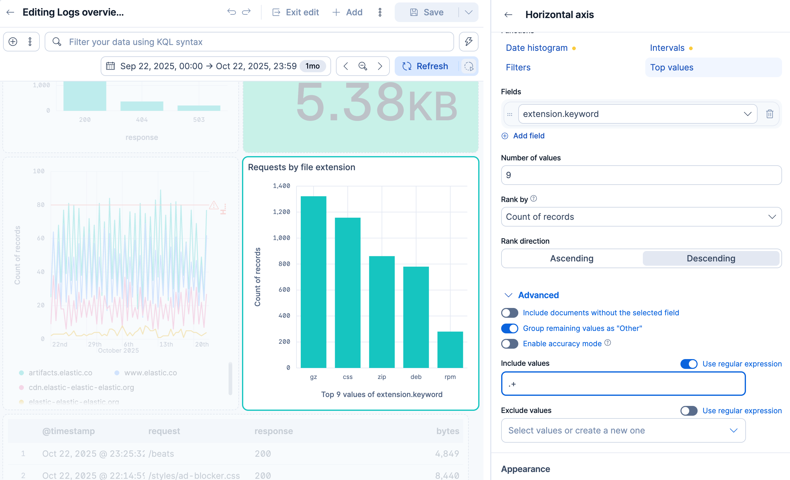
1. Hover over the panel and select Edit visualization. A Configuration flyout opens on the right side of the panel.
2. In the flyout, select the Horizontal axis configuration.
3. Expand Advanced, then in the Include values field, enter .+ and select Use regular expression. This regular expression matches any non-empty string, which filters out documents where the extension field is blank. The panel updates immediately to reflect the change.
4. Select Back, then Apply and close.
Tip

For more advanced editing, select Edit in Lens in the inline editing flyout to open the full Lens editor. When you are done, select Save and return to go back to the dashboard.
Try interactive filtering

Dashboard panels are interactive. Try selecting the 404 bar in the Events by response code chart. Kibana adds a filter for that value, and the other panels update to show only the matching log events. The metric, bar chart, and line chart now reflect only the 404 traffic.

To remove the filter, select the next to it in the dashboard's filter bar.

Tip

If you know which dimensions your viewers will want to filter by, you can add controls (dropdown menus, range sliders) directly to the dashboard so they don't have to build those filters themselves.
Arrange and save

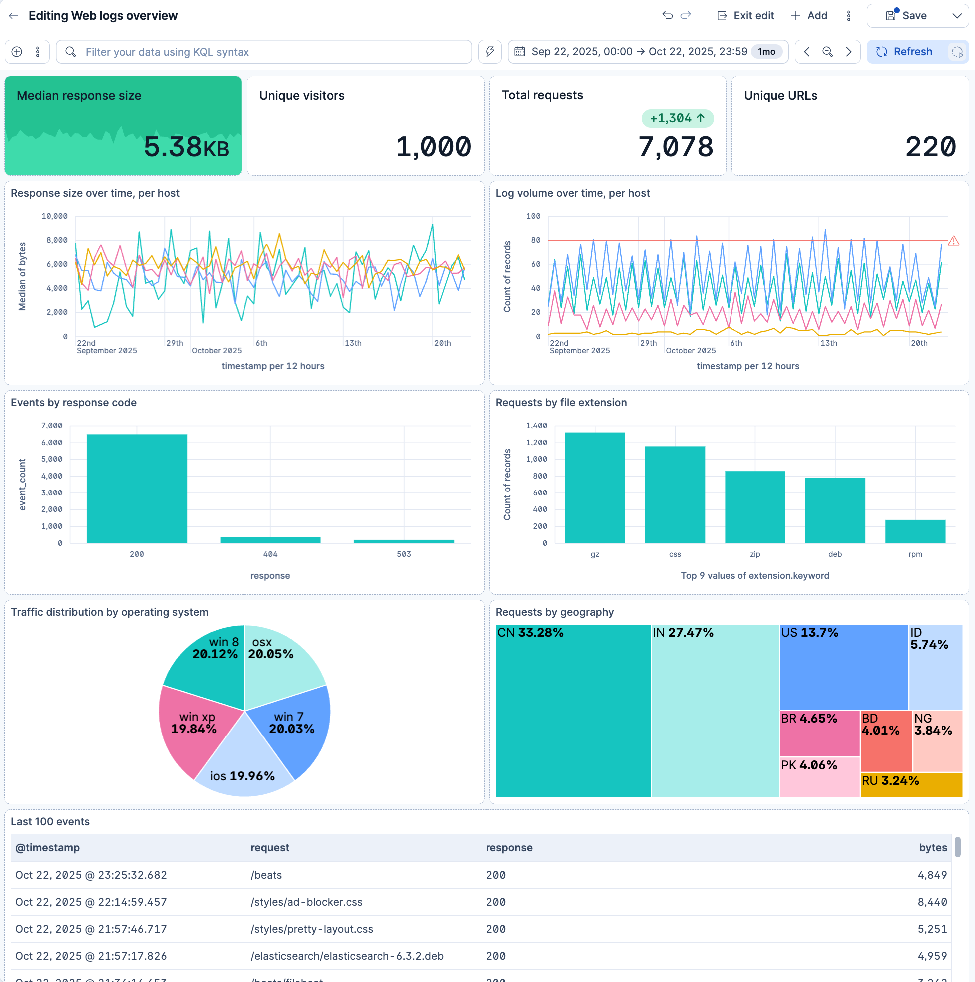
Drag panels by their header to reposition them, and drag the corner handles to resize them. A well-organized layout helps readers find what matters quickly. Aim for a compact, dense layout so the most important information is visible without scrolling:
- Top row: place metric panels side by side for key numbers at a glance. Keep them short, about 5 grid rows, so they don't dominate the page.
- Middle rows: arrange time series charts (line charts) and bar charts below the metrics. A moderate height (roughly 10–12 grid rows) gives charts enough room to be readable without wasting space.
- Bottom row: use wider panels for tables that benefit from more horizontal space and can afford a taller height.
For a panel sizing reference with recommended widths and heights for each chart type, refer to Organize dashboard panels.

To reduce clutter, consider hiding redundant axis titles. For example, on a bar chart the x-axis title may not add value when the panel title already describes the data. To hide it, edit the panel in Lens, open the Style panel, then under Bottom axis, set Axis title to None.

Tip

For larger dashboards, you can also group panels into collapsible sections to keep things organized.

When you are happy with the layout, select Save in the toolbar.

Your dashboard now combines multiple panel types built with Lens, and you've seen how inline editing and interactive filtering make the dashboard both customizable and interactive. To learn more, refer to Dashboards, Lens, and Panels and visualizations.

Once your dashboard is ready, share it with your team:

In the toolbar, select Share.
Copy the link and share it with your team.

Users who receive the link need to authenticate and have the appropriate privileges to access the underlying data.

Elastic Cloud Serverless projects are autoscaled environments, fully managed by Elastic and available on Elastic Cloud. Availability Generally available This functionality is generally available and ready for production usage. Serverless interfaces and procedures might differ from classic Elastic Stack deployments. The Elastic Stack includes Elastic's core products such as Elasticsearch, Kibana, Logstash, and Beats. Availability Generally available since 9.3 This functionality is generally available and ready for production usage. Unless stated otherwise on the page, this functionality is available when your Elastic Stack is deployed on Elastic Cloud Hosted, Elastic Cloud Enterprise, Elastic Cloud on Kubernetes, and self-managed environments. This documentation corresponds to the latest patch available for each minor version. If you're not using the latest patch, check the release notes for changes. From the same Share menu, you can also set whether other users in the space can edit or only view the dashboard. Users with view-only access can still duplicate it to create their own version.

For more details on sharing options, access control, and managing dashboard ownership, refer to Sharing dashboards.

Recreate the dashboard with the API

Everything you built in this tutorial can also be reproduced in a single API call. The Dashboards API accepts a JSON payload that encodes the complete dashboard, including panel types, data sources, layout, and display options, making it straightforward to version-control dashboards or provision consistent environments programmatically.

Recreate this dashboard with one API call

The following request creates the same dashboard as the one you built in this tutorial, including the optional panels suggestions.

Note

These API request examples are kept up to date with the latest version of the APIs, so some fields might differ if you're using an earlier version. For a history of breaking changes, refer to the Kibana breaking changes or the Elastic Cloud Serverless breaking changes.

Console

POST kbn://api/dashboards
{
  "title": "Web logs overview",
  "description": "Recreates the dashboard built in the Kibana data exploration tutorial.",
  "time_range": { "from": "now-90d", "to": "now" },
  "panels": [
    {
      "grid": { "x": 0, "y": 0, "w": 12, "h": 5 },
      "type": "vis",
      "config": {
        "type": "metric",
        "data_source": {
          "type": "data_view_spec",
          "index_pattern": "kibana_sample_data_logs",
          "time_field": "timestamp"
        },
        "metrics": [
          {
            "type": "primary",
            "operation": "median",
            "field": "bytes",
            "label": "Median response size",
            "format": { "type": "bytes", "decimals": 2 },
            "background_chart": { "type": "trend" },
            "color": {
              "type": "dynamic",
              "range": "absolute",
              "steps": [
                { "lt": 6000, "color": "#24c292" },
                { "gte": 6000, "lt": 10000, "color": "#fcd883" },
                { "gte": 10000, "color": "#f6726a" }
              ]
            },
            "apply_color_to": "background"
          }
        ]
      }
    },
    {
      "grid": { "x": 12, "y": 0, "w": 12, "h": 5 },
      "type": "vis",
      "config": {
        "type": "metric",
        "data_source": {
          "type": "data_view_spec",
          "index_pattern": "kibana_sample_data_logs",
          "time_field": "timestamp"
        },
        "metrics": [
          {
            "type": "primary",
            "operation": "unique_count",
            "field": "clientip",
            "label": "Unique visitors"
          }
        ]
      }
    },
    {
      "grid": { "x": 24, "y": 0, "w": 12, "h": 5 },
      "type": "vis",
      "config": {
        "type": "metric",
        "data_source": {
          "type": "data_view_spec",
          "index_pattern": "kibana_sample_data_logs",
          "time_field": "timestamp"
        },
        "metrics": [
          {
            "type": "primary",
            "operation": "count",
            "label": "Total requests"
          },
          {
            "type": "secondary",
            "operation": "count",
            "label": "Week to week",
            "time_shift": "1w",
            "compare": { "to": "primary", "palette": "compare_to", "icon": true, "value": true }
          }
        ]
      }
    },
    {
      "grid": { "x": 36, "y": 0, "w": 12, "h": 5 },
      "type": "vis",
      "config": {
        "type": "metric",
        "data_source": {
          "type": "data_view_spec",
          "index_pattern": "kibana_sample_data_logs",
          "time_field": "timestamp"
        },
        "metrics": [
          {
            "type": "primary",
            "operation": "unique_count",
            "field": "request.keyword",
            "label": "Unique URLs"
          }
        ]
      }
    },
    {
      "grid": { "x": 0, "y": 5, "w": 24, "h": 10 },
      "type": "vis",
      "config": {
        "type": "xy",
        "title": "Response size over time, per host",
        "layers": [
          {
            "type": "line",
            "data_source": {
              "type": "data_view_spec",
              "index_pattern": "kibana_sample_data_logs",
              "time_field": "timestamp"
            },
            "x": { "operation": "date_histogram", "field": "timestamp" },
            "y": [{ "operation": "median", "field": "bytes" }],
            "breakdown_by": {
              "operation": "terms",
              "fields": ["host.keyword"],
              "limit": 9
            }
          }
        ]
      }
    },
    {
      "grid": { "x": 24, "y": 5, "w": 24, "h": 10 },
      "type": "vis",
      "config": {
        "type": "xy",
        "title": "Log volume over time, per host",
        "layers": [
          {
            "type": "line",
            "data_source": {
              "type": "data_view_spec",
              "index_pattern": "kibana_sample_data_logs",
              "time_field": "timestamp"
            },
            "x": { "operation": "date_histogram", "field": "timestamp" },
            "y": [{ "operation": "count" }],
            "breakdown_by": {
              "operation": "terms",
              "fields": ["host.keyword"],
              "limit": 9
            }
          },
          {
            "type": "reference_lines",
            "data_source": {
              "type": "data_view_spec",
              "index_pattern": "kibana_sample_data_logs",
              "time_field": "timestamp"
            },
            "thresholds": [
              {
                "operation": "static_value",
                "value": 80,
                "label": "High traffic",
                "color": { "type": "static", "color": "#f6726a" },
                "icon": "alert"
              }
            ]
          }
        ]
      }
    },
    {
      "grid": { "x": 0, "y": 15, "w": 24, "h": 10 },
      "type": "vis",
      "config": {
        "type": "xy",
        "title": "Events by response code",
        "layers": [
          {
            "type": "bar_stacked",
            "data_source": {
              "type": "esql",
              "query": "FROM kibana_sample_data_logs | WHERE response IS NOT NULL | STATS event_count = COUNT(*) BY response | SORT event_count DESC | LIMIT 50"
            },
            "x": { "column": "response" },
            "y": [{ "column": "event_count" }]
          }
        ]
      }
    },
    {
      "grid": { "x": 24, "y": 15, "w": 24, "h": 10 },
      "type": "vis",
      "config": {
        "type": "xy",
        "title": "Requests by file extension",
        "layers": [
          {
            "type": "bar_stacked",
            "data_source": {
              "type": "data_view_spec",
              "index_pattern": "kibana_sample_data_logs",
              "time_field": "timestamp"
            },
            "x": {
              "operation": "terms",
              "fields": ["extension.keyword"],
              "limit": 9,
              "includes": { "as_regex": true, "values": [".+"] }
            },
            "y": [{ "operation": "count" }]
          }
        ]
      }
    },
    {
      "grid": { "x": 0, "y": 25, "w": 24, "h": 10 },
      "type": "vis",
      "config": {
        "type": "pie",
        "title": "Traffic distribution by operating system",
        "data_source": {
          "type": "data_view_spec",
          "index_pattern": "kibana_sample_data_logs",
          "time_field": "timestamp"
        },
        "metrics": [{ "operation": "count" }],
        "group_by": [
          {
            "operation": "terms",
            "fields": ["machine.os.keyword"],
            "limit": 9
          }
        ]
      }
    },
    {
      "grid": { "x": 24, "y": 25, "w": 24, "h": 10 },
      "type": "vis",
      "config": {
        "type": "treemap",
        "title": "Requests by geography",
        "data_source": {
          "type": "data_view_spec",
          "index_pattern": "kibana_sample_data_logs",
          "time_field": "timestamp"
        },
        "metrics": [{ "operation": "count" }],
        "group_by": [
          {
            "operation": "terms",
            "fields": ["geo.dest"],
            "limit": 9
          }
        ]
      }
    },
    {
      "grid": { "x": 0, "y": 35, "w": 48, "h": 17 },
      "type": "vis",
      "config": {
        "type": "data_table",
        "title": "Last 100 events",
        "data_source": {
          "type": "esql",
          "query": "FROM kibana_sample_data_logs | KEEP @timestamp, request, response, bytes | SORT @timestamp DESC | LIMIT 100"
        },
        "rows": [
          { "column": "@timestamp" },
          { "column": "request" },
          { "column": "response" }
        ],
        "metrics": [
          { "column": "bytes" }
        ]
      }
    }
  ]
}

How each panel maps back to the tutorial:

Median response size: Lens metric panel from the Add a metric panel for median response size sub-step, including the bytes format, the trend background_chart for the sparkline, and the dynamic color thresholds.
Unique visitors: unique_count of clientip, from the Optional: add more metrics to build a row suggestion.
Total requests: count with a secondary metric configured for week-over-week comparison via time_shift: "1w" and compare. Same source as the unique-visitors suggestion.
Unique URLs: unique_count of request.keyword, also from the optional metrics row.
Response size over time, per host: line chart of median bytes split by host, from the Optional: add more time series suggestion in the line-chart sub-step.
Log volume over time, per host: the line chart from the Add a line chart of log volume over time sub-step. The reference line at value 80 is a separate reference_lines layer in the same panel.
Events by response code: the ES|QL bar chart saved to the dashboard from Discover in Step 2. ES|QL chart layers reference query result columns directly in x and y (for example, "x": { "column": "response" }), instead of the operation-based form used by data view layers.
Requests by file extension: bar chart from the Add a bar chart of requests by file extension sub-step. The includes filter with as_regex: true and value .+ mirrors the regex applied during the inline-edit step.
Traffic distribution by operating system: pie chart from the Expand your dashboard sub-step. Pie panels use config.type: "pie" with a metrics array and a group_by array.
Requests by geography: treemap from the same sub-step. Treemaps use the same metrics + group_by shape as pies.
Last 100 events: ES|QL data table from the Add a table of recent events with ES|QL sub-step. Categorical columns go in rows, numeric columns go in metrics.

curl

curl -X POST "${KIBANA_URL}/api/dashboards" \
  -H "Authorization: ApiKey ${API_KEY}" \
  -H "kbn-xsrf: true" \
  -H "Content-Type: application/json" \
  -d '{
  "title": "Web logs overview",
  "description": "Recreates the dashboard built in the Kibana data exploration tutorial.",
  "time_range": { "from": "now-90d", "to": "now" },
  "panels": [
    {
      "grid": { "x": 0, "y": 0, "w": 12, "h": 5 },
      "type": "vis",
      "config": {
        "type": "metric",
        "data_source": {
          "type": "data_view_spec",
          "index_pattern": "kibana_sample_data_logs",
          "time_field": "timestamp"
        },
        "metrics": [
          {
            "type": "primary",
            "operation": "median",
            "field": "bytes",
            "label": "Median response size",
            "format": { "type": "bytes", "decimals": 2 },
            "background_chart": { "type": "trend" },
            "color": {
              "type": "dynamic",
              "range": "absolute",
              "steps": [
                { "lt": 6000, "color": "#24c292" },
                { "gte": 6000, "lt": 10000, "color": "#fcd883" },
                { "gte": 10000, "color": "#f6726a" }
              ]
            },
            "apply_color_to": "background"
          }
        ]
      }
    },
    {
      "grid": { "x": 12, "y": 0, "w": 12, "h": 5 },
      "type": "vis",
      "config": {
        "type": "metric",
        "data_source": {
          "type": "data_view_spec",
          "index_pattern": "kibana_sample_data_logs",
          "time_field": "timestamp"
        },
        "metrics": [
          {
            "type": "primary",
            "operation": "unique_count",
            "field": "clientip",
            "label": "Unique visitors"
          }
        ]
      }
    },
    {
      "grid": { "x": 24, "y": 0, "w": 12, "h": 5 },
      "type": "vis",
      "config": {
        "type": "metric",
        "data_source": {
          "type": "data_view_spec",
          "index_pattern": "kibana_sample_data_logs",
          "time_field": "timestamp"
        },
        "metrics": [
          {
            "type": "primary",
            "operation": "count",
            "label": "Total requests"
          },
          {
            "type": "secondary",
            "operation": "count",
            "label": "Week to week",
            "time_shift": "1w",
            "compare": { "to": "primary", "palette": "compare_to", "icon": true, "value": true }
          }
        ]
      }
    },
    {
      "grid": { "x": 36, "y": 0, "w": 12, "h": 5 },
      "type": "vis",
      "config": {
        "type": "metric",
        "data_source": {
          "type": "data_view_spec",
          "index_pattern": "kibana_sample_data_logs",
          "time_field": "timestamp"
        },
        "metrics": [
          {
            "type": "primary",
            "operation": "unique_count",
            "field": "request.keyword",
            "label": "Unique URLs"
          }
        ]
      }
    },
    {
      "grid": { "x": 0, "y": 5, "w": 24, "h": 10 },
      "type": "vis",
      "config": {
        "type": "xy",
        "title": "Response size over time, per host",
        "layers": [
          {
            "type": "line",
            "data_source": {
              "type": "data_view_spec",
              "index_pattern": "kibana_sample_data_logs",
              "time_field": "timestamp"
            },
            "x": { "operation": "date_histogram", "field": "timestamp" },
            "y": [{ "operation": "median", "field": "bytes" }],
            "breakdown_by": {
              "operation": "terms",
              "fields": ["host.keyword"],
              "limit": 9
            }
          }
        ]
      }
    },
    {
      "grid": { "x": 24, "y": 5, "w": 24, "h": 10 },
      "type": "vis",
      "config": {
        "type": "xy",
        "title": "Log volume over time, per host",
        "layers": [
          {
            "type": "line",
            "data_source": {
              "type": "data_view_spec",
              "index_pattern": "kibana_sample_data_logs",
              "time_field": "timestamp"
            },
            "x": { "operation": "date_histogram", "field": "timestamp" },
            "y": [{ "operation": "count" }],
            "breakdown_by": {
              "operation": "terms",
              "fields": ["host.keyword"],
              "limit": 9
            }
          },
          {
            "type": "reference_lines",
            "data_source": {
              "type": "data_view_spec",
              "index_pattern": "kibana_sample_data_logs",
              "time_field": "timestamp"
            },
            "thresholds": [
              {
                "operation": "static_value",
                "value": 80,
                "label": "High traffic",
                "color": { "type": "static", "color": "#f6726a" },
                "icon": "alert"
              }
            ]
          }
        ]
      }
    },
    {
      "grid": { "x": 0, "y": 15, "w": 24, "h": 10 },
      "type": "vis",
      "config": {
        "type": "xy",
        "title": "Events by response code",
        "layers": [
          {
            "type": "bar_stacked",
            "data_source": {
              "type": "esql",
              "query": "FROM kibana_sample_data_logs | WHERE response IS NOT NULL | STATS event_count = COUNT(*) BY response | SORT event_count DESC | LIMIT 50"
            },
            "x": { "column": "response" },
            "y": [{ "column": "event_count" }]
          }
        ]
      }
    },
    {
      "grid": { "x": 24, "y": 15, "w": 24, "h": 10 },
      "type": "vis",
      "config": {
        "type": "xy",
        "title": "Requests by file extension",
        "layers": [
          {
            "type": "bar_stacked",
            "data_source": {
              "type": "data_view_spec",
              "index_pattern": "kibana_sample_data_logs",
              "time_field": "timestamp"
            },
            "x": {
              "operation": "terms",
              "fields": ["extension.keyword"],
              "limit": 9,
              "includes": { "as_regex": true, "values": [".+"] }
            },
            "y": [{ "operation": "count" }]
          }
        ]
      }
    },
    {
      "grid": { "x": 0, "y": 25, "w": 24, "h": 10 },
      "type": "vis",
      "config": {
        "type": "pie",
        "title": "Traffic distribution by operating system",
        "data_source": {
          "type": "data_view_spec",
          "index_pattern": "kibana_sample_data_logs",
          "time_field": "timestamp"
        },
        "metrics": [{ "operation": "count" }],
        "group_by": [
          {
            "operation": "terms",
            "fields": ["machine.os.keyword"],
            "limit": 9
          }
        ]
      }
    },
    {
      "grid": { "x": 24, "y": 25, "w": 24, "h": 10 },
      "type": "vis",
      "config": {
        "type": "treemap",
        "title": "Requests by geography",
        "data_source": {
          "type": "data_view_spec",
          "index_pattern": "kibana_sample_data_logs",
          "time_field": "timestamp"
        },
        "metrics": [{ "operation": "count" }],
        "group_by": [
          {
            "operation": "terms",
            "fields": ["geo.dest"],
            "limit": 9
          }
        ]
      }
    },
    {
      "grid": { "x": 0, "y": 35, "w": 48, "h": 17 },
      "type": "vis",
      "config": {
        "type": "data_table",
        "title": "Last 100 events",
        "data_source": {
          "type": "esql",
          "query": "FROM kibana_sample_data_logs | KEEP @timestamp, request, response, bytes | SORT @timestamp DESC | LIMIT 100"
        },
        "rows": [
          { "column": "@timestamp" },
          { "column": "request" },
          { "column": "response" }
        ],
        "metrics": [
          { "column": "bytes" }
        ]
      }
    }
  ]
}'

How each panel maps back to the tutorial:

Median response size: Lens metric panel from the Add a metric panel for median response size sub-step, including the bytes format, the trend background_chart for the sparkline, and the dynamic color thresholds.
Unique visitors: unique_count of clientip, from the Optional: add more metrics to build a row suggestion.
Total requests: count with a secondary metric configured for week-over-week comparison via time_shift: "1w" and compare. Same source as the unique-visitors suggestion.
Unique URLs: unique_count of request.keyword, also from the optional metrics row.
Response size over time, per host: line chart of median bytes split by host, from the Optional: add more time series suggestion in the line-chart sub-step.
Log volume over time, per host: the line chart from the Add a line chart of log volume over time sub-step. The reference line at value 80 is a separate reference_lines layer in the same panel.
Events by response code: the ES|QL bar chart saved to the dashboard from Discover in Step 2. ES|QL chart layers reference query result columns directly in x and y (for example, "x": { "column": "response" }), instead of the operation-based form used by data view layers.
Requests by file extension: bar chart from the Add a bar chart of requests by file extension sub-step. The includes filter with as_regex: true and value .+ mirrors the regex applied during the inline-edit step.
Traffic distribution by operating system: pie chart from the Expand your dashboard sub-step. Pie panels use config.type: "pie" with a metrics array and a group_by array.
Requests by geography: treemap from the same sub-step. Treemaps use the same metrics + group_by shape as pies.
Last 100 events: ES|QL data table from the Add a table of recent events with ES|QL sub-step. Categorical columns go in rows, numeric columns go in metrics.

For the full request schema, including sections, filter controls, and library-linked panels, refer to the Dashboards API reference.

Navigate between Discover and dashboards

One of Kibana's strengths is how you can move between exploring raw data and visualizing it. Here are the key navigation paths:

From Discover to a dashboard: When an ES|QL aggregation produces a chart in Discover, select Save visualization to dashboard (or Save visualization in earlier versions) next to the chart, then select Add to dashboard to send it to an existing or new dashboard. In classic mode, the chart has no save button. Select Edit visualization to open the chart in Lens, then save it from there, as Add Discover visualizations to dashboards describes. You can also save the current view of the table to a dashboard from the Discover table toolbar, or save the entire Discover session to the library and add it as a panel from a dashboard.
From a dashboard panel back to Discover: Open the context menu on any Lens panel and select Explore in Discover. Kibana opens Discover with the panel's query and filters already applied, so you can drill into the underlying data.
Inline and full Lens editing from a dashboard: Select on any panel to open the inline Configuration flyout. For deeper changes, select Edit in Lens in the flyout to switch to the full editor, then Save and return to go back to the dashboard.
Add a new visualization directly from a dashboard: From a dashboard, select Add, then select Create visualization (Visualization in earlier versions) to open the Lens editor, or Create visualization (query) (Visualization (query) in earlier versions) to create a chart from an ES|QL query without going through Discover first.

Tip

This back-and-forth workflow is especially useful when investigating anomalies: spot something unusual on a dashboard, jump to Discover to examine the raw events, refine your query, then save an updated visualization back to the dashboard.

Next steps

You've completed the core workflow, from sample data to a shareable dashboard. Here are some directions to explore next:

Bring in your own data : The same workflow applies to any data in Elasticsearch. Use Elastic Agent to ingest your own logs, metrics, or traces. Refer to Ingest data for an overview of all ingestion options.

Deepen your ES|QL knowledge : ES|QL supports advanced operations like ENRICH, LOOKUP JOIN, DISSECT, and GROK, and more to transform your data on the fly. Refer to the ES|QL reference and Use ES|QL in Kibana.

Explore different types of data : Depending on what you monitor, you can use specialized tools:

Logs: Explore logs in Discover with field-level filtering and log parsing.
Metrics: Get started with system metrics and the Infrastructure app.
Traces: Get started with APM to trace requests across distributed services.

Try more visualization techniques : Build richer dashboards with the following step-by-step tutorials:

Add geographic context : The sample web logs data includes geo.src and geo.dest fields. Maps lets you visualize this data on interactive maps and add them to dashboards.

Set up alerts : Don't wait for problems to show up on a dashboard. Create alerting rules to get notified when your data crosses a threshold.

Try machine learning : Use machine learning to detect anomalies in time-series data, forecast trends, or categorize log messages. The sample data sets include pre-configured anomaly detection jobs you can experiment with.