Detect change points in Discover

If a metric suddenly jumped, dropped, or changed its trend, you can find out when it happened. A CHANGE_POINT query in Discover detects statistically significant changes in time series data, such as spikes, dips, and shifts in distribution or trend. Discover charts each analyzed series, which is one metric over time, and marks the changes it finds. The results table stays available for investigation. Discover shows the charts 8 at a time, so use the pagination controls to move between pages when your query returns more series.

• Make sure Discover is in ES|QL mode. Classic mode doesn't support this functionality. To switch, refer to Switch to Discover's ES|QL mode.
• You need a Platinum or Enterprise subscription or an active trial for Elastic Stack. On Elastic Cloud Serverless, CHANGE_POINT is available for all project types, except Observability projects on the Logs Essentials tier.
• To analyze your own data, you need a date field and values that you can aggregate into a numeric metric. The CHANGE_POINT command requires at least 22 values per series, and it analyzes only the first 1,000 values of each series.
• To follow the example, add the Sample web logs data.

In this example, you use the sample web logs data to detect changes in the average number of bytes transferred for each destination country.

1. Open Discover. Find it in the navigation menu or use the global search field.

2. Set the time range to cover about 60 days of the sample data. The sample data is shifted around the day you add it, so it spans roughly the 10 days before that day and the 50 days after it. A range that ends at now, such as Last 30 days, leaves out most of the data and gives too few values. To set the range:

   1. In the time filter, select the start date. On the Relative tab, enter 15 and select Days ago.
   2. Select the end date. On the Relative tab, enter 60 and select Days from now.

3. Enter the following query:

   FROM kibana_sample_data_logs
   | STATS avg_bytes = AVG(bytes) BY geo.dest, day = BUCKET(@timestamp, 1d)
   | CHANGE_POINT avg_bytes ON day BY geo.dest
   | WHERE type IS NOT NULL
   

   The query calculates the average number of bytes transferred each day for every destination country, then returns the detected change points.

4. Select Search.

   Discover shows a separate chart for each destination country with a detected change point. The results table lists the detected changes. The p-value measures the statistical significance of a change point. Lower values indicate a more significant change.

   
   

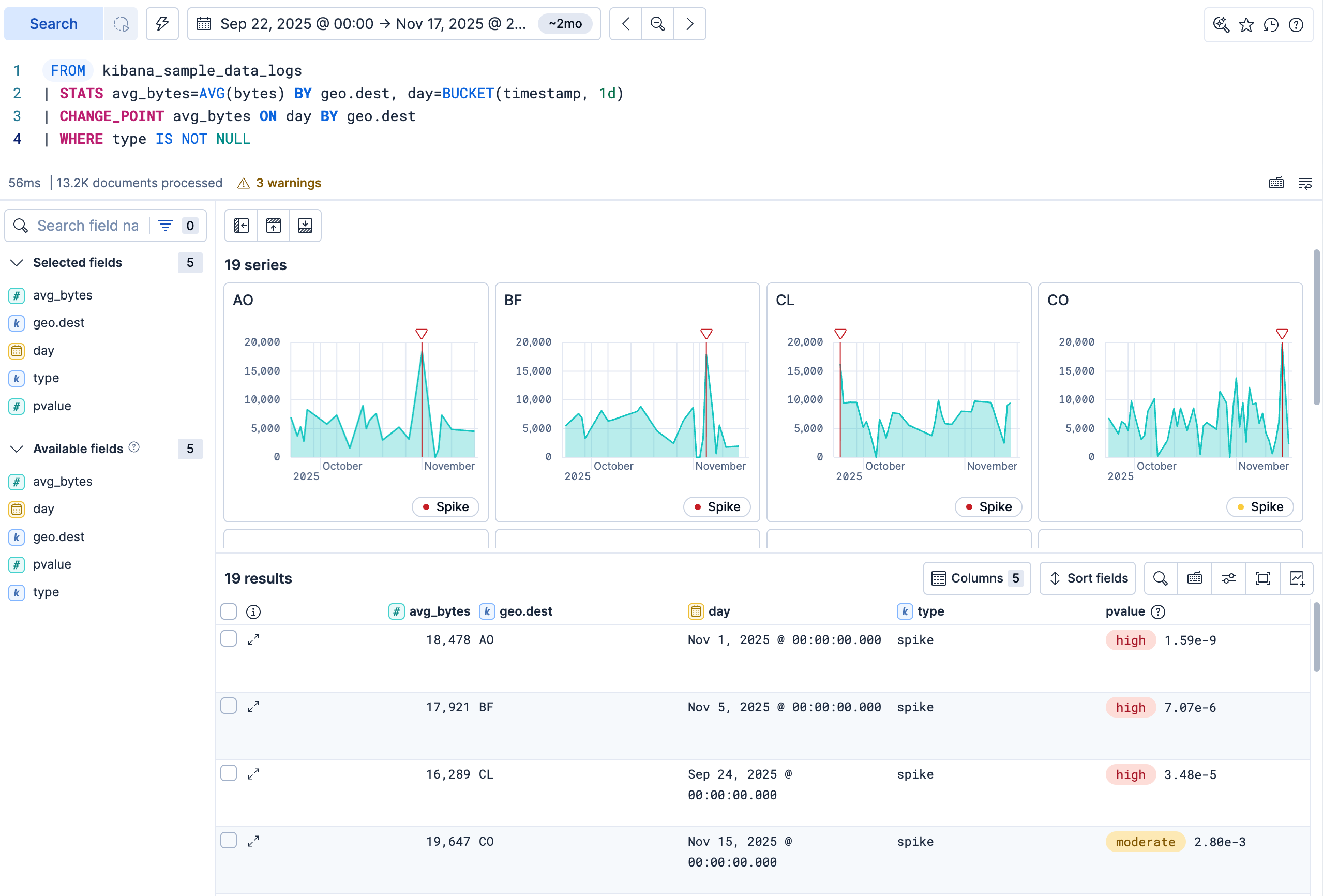
To investigate the results further, you can:

• Attach a chart to a case: Hover over the chart and select Add to case. Then select an existing case or create a case. You need the All Cases privilege to use this action.

• Inspect a change point: Expand a change point in the results table. The Overview tab shows its chart, plus the time, field, metric, change point type, p-value, and a description. Next to the p-value, a high, moderate, or low badge shows how significant the change is.

• Look at one change in detail: From the chart actions, select Open in a new Discover tab to open the series in a focused time range around the detected change. For queries that read from an index, the new tab shows the source documents.

  
  

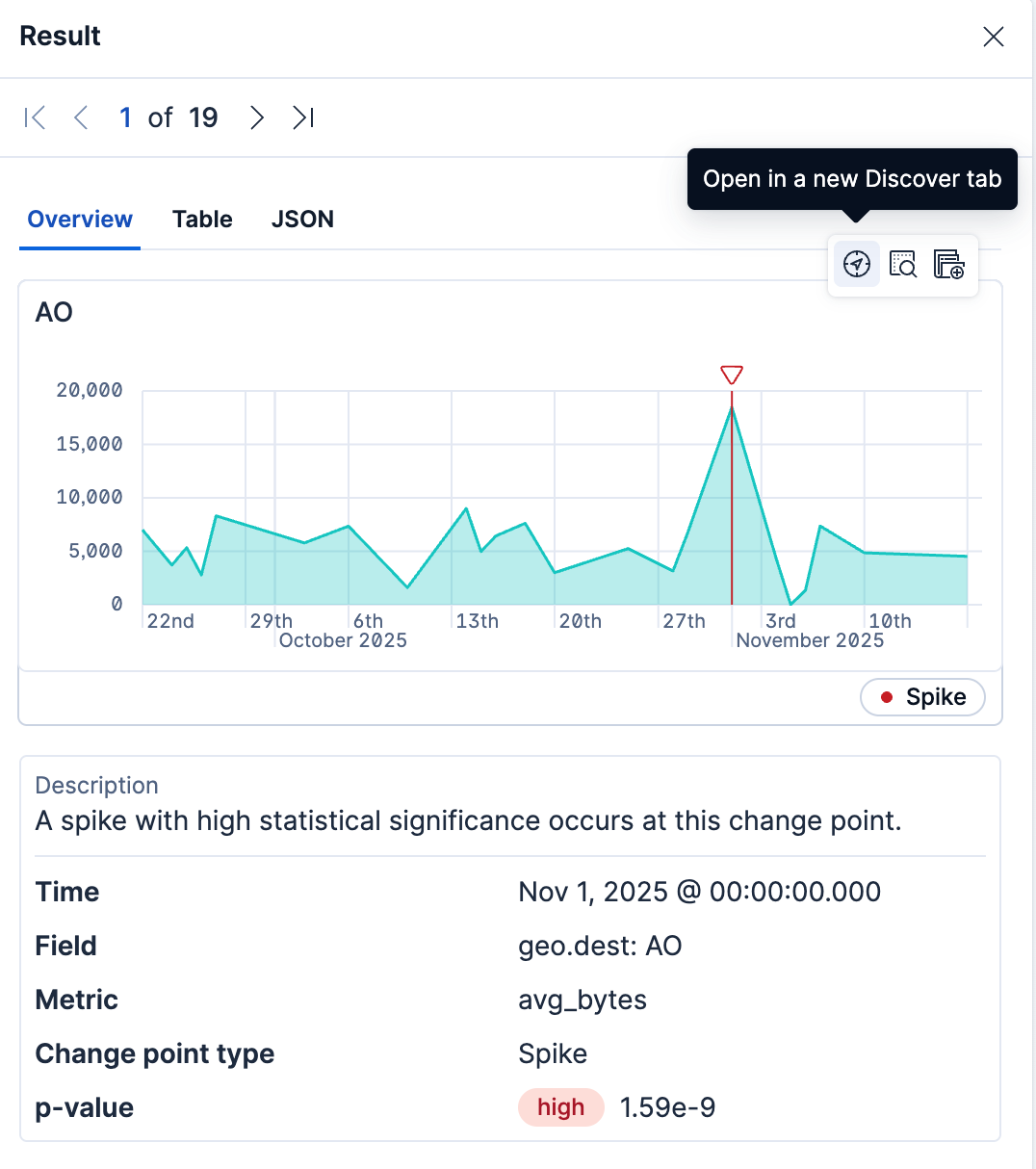
• Save the session: Save the Discover session to preserve the query and time range.

Structure your query so that it produces one numeric metric value per time bucket before calling CHANGE_POINT. For example, the following query analyzes changes in log volume over the selected time range:

FROM logs-*
| WHERE @timestamp <= ?_tend AND @timestamp > ?_tstart
| STATS event_count = COUNT(*) BY time_bucket = BUCKET(@timestamp, 50, ?_tstart, ?_tend)
| SORT time_bucket
| CHANGE_POINT event_count ON time_bucket
| WHERE type IS NOT NULL

• Adapt the query to your data: Replace the index, time field, and aggregation with values appropriate for your data.
• If no change points are detected: The data either has no statistically significant change or doesn't provide the 22 values required for analysis. Widen the time range or adjust the bucket size to provide more values.
• If your series is long: Only the first 1,000 values of each series are analyzed. Use larger time buckets so that each series stays under that limit.

Add fields to BY to analyze each unique combination as a separate series. For example, the following query analyzes the sum of transferred bytes for each host and response code in the sample web logs data:

FROM kibana_sample_data_logs
| STATS sum_bytes = SUM(bytes) BY host, response.keyword, day = BUCKET(@timestamp, 1d)
| CHANGE_POINT sum_bytes ON day BY host, response.keyword
| WHERE type IS NOT NULL

Discover displays a separate chart for each group that contains a detected change point. Use the chart grid to compare where each series changed.

• Get started with ES|QL in Discover
• How to query in Discover's ES|QL mode
• CHANGE_POINT command reference
• Detect change points in AIOps Labs